Abstract
For the first time, a new continuous distribution, called the generalized beta exponentiated Pareto type I (GBEP) [McDonald exponentiated Pareto] distribution, is defined and investigated. The new distribution contains as special sub-models some well-known and not known distributions, such as the generalized beta Pareto (GBP) [McDonald Pareto], the Kumaraswamy exponentiated Pareto (KEP), Kumaraswamy Pareto (KP), beta exponentiated Pareto (BEP), beta Pareto (BP), exponentiated Pareto (EP) and Pareto, among several others. Various structural properties of the new distribution are derived, including explicit expressions for the moments, moment generating function, incomplete moments, quantile function, mean deviations and Rényi entropy. Lorenz, Bonferroni and Zenga curves are derived. The method of maximum likelihood is proposed for estimating the model parameters. We obtain the observed information matrix. The usefulness of the new model is illustrated by means of two real data sets. We hope that this generalization may attract wider applications in reliability, biology and lifetime data analysis.
Keywords: Beta-Generated class; Pareto type I distribution; Lorenz, Bonferroni and Zenga curves; Rényi entropy; Maximum likelihood estimation.
1. Introduction
The Pareto distribution named after the Italian economist Vilfredo Pareto (1848-1923) is a power law probability distribution that coincides with social, scientific, geophysical, actuarial, and many other types of observable phenomena. Outside the field of economics it is at times referred to as the Bradford distribution. Burroughs and Tebbens (2001) discussed applications of the Pareto distribution in modeling earthquakes, forest fire areas and oil and gas field sizes and Schroeder et al. (2010) presented an application of the Pareto distribution in modeling disk drive sector errors. To add flexibility to the Pareto distribution, various generalizations of the distribution have been derived, the beta Pareto distribution discussed by Akinsete et al. (2008), the Kumaraswamy Pareto distribution introduced by Bourguignon et al. (2013), the beta generalized Pareto defined by Nassar and Nada (2011) and Mahmoudi (2011), the beta exponentiated Pareto distribution presented by Zea et al. (2012), the gamma Pareto distribution introduced by Alzaatreh et al. (2012) and recently, ElbataL (2013) studied the Kumaraswamy exponentiated Pareto distribution.
The cdf of the exponentiated Pareto type I distribution with parameters , k and d is
given by
( ; , , ) 1 ( )k ,
G x d k d x (1)
where 0,d0,k 0 and
x
d
. The corresponding pdf is given by1 ( 1)
( ; , , ) k k 1 ( )k .
g x d k k d x d x (2) M. E. Mead
Department of Statistics and Insurance
Faculty of Commerce, Zagazig University, Egypt
Eugene et al. (2002) used the beta distribution as a generator to develop the so-called family of beta-generated distributions (BG). The cdf of a beta-generated random variable
X is defined as
( )
1 1
( )
0
1
( ; , ) ( , ) (1 ) ,
( , ) G x
a b
G x
F x a b I a b w w dw
B a b
(3)
for a0, b0, where I a by( , )B a b B a by( , ) ( , ) denotes the incomplete beta function
ratio of type I and 1 1
0
( , ) y a (1 )b y
B a b
w w dw is the incomplete beta function. The pdf corresponding to (3) can be expressed as
11
1
( ; , ) ( ) ( ) 1 ( ) ,
( , )
b a
f x a b g x G x G x
B a b
(4)
where g x( ) G x( ) x is the baseline density function.
Eugene et al. (2002) has used the cdf of normal distribution in (4) to construct the beta normal distribution. The generalization given in (4) has been used by number of authors to propose new distributions. This family of distributions is a generalization of the distributions of order statistics for the random variableXwith cdf F x( ) as pointed out by
Eugene et al. (2002) and Jones (2004). Since the paper by Eugene et al. (2002), many beta-generated distributions have been studied in the literature including, beta gamma distribution by Kong et al. (2007), beta Weibull distribution by Famoye et al. (2005), beta exponential distribution by Nadarajah and Kotz (2006) and others.
Cordeiro and de Castro (2011) extended the beta-generated family of distributions by replacing the beta distribution in (3) with the Kumaraswamy distribution (1980),
1 1
( ) a (1 a b) , 0 1.
g x abx x x The cdf of the Kumaraswamy generalized distributions
(KG) is given by
( ; , ) 1 1 ( )c b
F x b c G x (5)
and the corresponding pdf is defined as
1 1
( ; , ) ( ) ( )c 1 ( )c b .
f x b c cb g x G x G x (6)
Several generalized distributions from (6) have been defined and investigated in the literature including the Kumaraswamy Weibull distribution by Cordeiro et al. (2010), the Kumaraswamy generalized gamma distribution by de Castro et al. (2011) and the Kumaraswamy generalized half-normal distribution by Cordeiro et al. (2012).
Kumaraswamy-generated (KG) and exponentiated distributions. They defined the cdf of the GBG as the form
( )
1 1
0
( )
1
( ; , , ) (1 )
( , ) ( , )
c
c G x
a b
G x
F x a b c w w dw
B a b
I a b
(7)and the corresponding pdf is given by
1 1
( ; , , ) ( ) ( ) 1 ( ) .
( , )
b
a c c
c
f x a b c g x G x G x
B a b
(8)
The importance of the density(8) is that it contains as special sub-models, the BG (c1),
the KG (a1)and the exponentiated (b c 1) distributions .The generalization given in (8) has been used by number of authors including Marciano et al. (2012), Corderio et al. (2014), Oluyede and Rajasooriya (2013) and Tahir et al. (2014).
2. Generalized Beta Exponentiated Pareto Distribution
In this note we propose the generalized beta exponentiated Pareto (GBEP) distribution by using the density function (2) in (8). The pdf of GBEP can be expressed as
( 1) 1 1
( ; ) 1 ( ) 1 1 ( ) ,
( , )
k k a c c b
k k
c k d x
f x d x d x
B a b
(9)
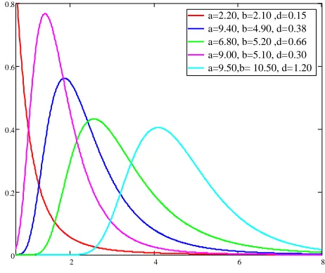
where ( , , , , , )a b d k c is the vector of the model parameters. Plots of the GBEP for selected parameter values (c1.4, 2.3&k 1.2 and different values ofa b, &d) are given in Figure 1.
2 4 6 8
0 0.2 0.4 0.6 0.8
a=2.20, b=2.10 ,d=0.15 a=9.40, b=4.90, d=0.38 a=6.80, b=5.20 ,d=0.66 a=9.00, b=5.10, d=0.30 a=9.50,b= 10.50, d=1.20
Figure 1: Some possible shapes of the GBEP density function The cdf corresponding to (9) is
1 ( )
( ; ) k c ( , ). d x
F x I a b
Equation (10) can be expressed as follows
2 1
1 ( )
( ; ) ,1 ; 1; 1 ( ) ,
( , ) a c k
c k d x
F x F a b a d x
a B a b
(11)
where
1 1 12 1
0
1 (1 )
, ; ; ,
( , ) (1 )
b c b
a
t t
F a b c z dt
B b c b t z
is the well known hypergeometric function (Gradshteyn and Ryzhik, 2007).
For a lifetime random variable t, the survival function S(t), hazard rate function h(t),
reversed hazard rate function r (t) and the cumulative hazard rate function H(t) of GBEP distribution are given by
1 ( )
( ) 1 ( ) 1 k c ( , ),
d t
S t F t I a b
1 1
11 ( )
1 ( ) 1 1 ( )
( )
( ) ,
( )
( , ) k c ( , )
b c a c
k
k k k
d t
c k d t d t d t
f t h t
S t
B a b B a b
11 ( 1)
1 ( )
1 ( ) 1 1 ( )
( ) ( )
( ) k c ( , )
b c a c
k k k k
d t
c k d t d t d t
f t r t
F t B a b
and
1 ( )
( ) ( ) 1 k c ( , )
d t
H t n S t n I a b
.
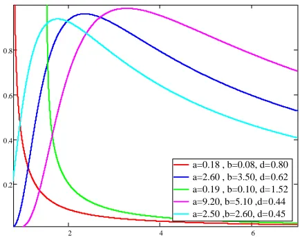
Plots of the hazard rate function (HRF) for selected parameter values (c1.4, 2.3 &k 1.2and different values of a b, & d) are given in Figure 2.
2 4 6
0.2 0.4 0.6 0.8
a=0.18 , b=0.08, d=0.80 a=2.60 , b=3.50, d=0.62 a=0.19 , b=0.10, d=1.52 a=9.20, b=5.10 ,d=0.44 a=2.50 ,b=2.60, d=0.45
Note that the GBEP distribution has several well known models as special cases, which make it of distinguishable scientific importance from other distributions.
1. The study of the new density (9) is important, since it includes as special sub-models some distributions not previously considered in the literature. Setting
1
, the density (9) gives the generalized beta Pareto (GBP) [also known as the McDonald Pareto type I] distribution.
2. If a1,equation (9) reduces to Kumaraswamy exponentiated Pareto (KEP) distribution defined by Elbatal (2013).
3. Setting c1, the density (9) gives the beta exponentiated Pareto (BEP) distribution presented by Zea et al. (2012) and the beta generalized Pareto defined by Nassar and Nada (2011).
4. If a 1,equation (9) corresponds to the Kumaraswamy Pareto (KP) distribution introduced by Bourguignon et al. (2013).
5. Setting c 1, GBEP becomes the beta Pareto (BP) distribution discussed by Akinsete et al. (2008).
6. When a b c 1,the density (9) corresponds to the exponentiated Pareto (EP) [also known as Stoppa or the generalized Pareto type I] distribution defined by Gupta et al. (1998).
7. If we takea b c 1, equation (9) becomes the Pareto (P) distribution.
3. Some Statistical Properties
We give a mathematical treatment of the new distribution including expansions of the GBEP cdf and pdf, moments, incomplete moments, generating and quantile functions, mean deviations, mean residual life, Lorenz, Bonferroni and Zenga curves and Rényi entropy.
3.1 Expansion of Distribution
We now present a series expansion of the GBEP cdf and pdf. For any positive real number b, and for |z| < 1, a generalized binomial expansion holds
10
( 1) ( )
1 .
! ( )
j
b j
j
b
z z
j b j
Therefore, the cdf of GBEP can be expanded to obtain
1
1 0 0
0
1 ( 1) ( )
;
( , ) ! ( )
( ; , , ( )),
c k
d x
j a j
j j
j
b
F x w dw
B a b j b j
p G x d k c a j
(12)
where
( 1) ( )
( ) ! ( )( )
j j
a b p
a j b j a j
and G x d k( ; , ,c a( j)) denotes the cdf of EP with parametersd, k and c a( j). Similarly, we can write the pdf (9) as
( ) 1( 1) 0
0
( )( 1)
; 1
( ) ! ( )
( ; , , ( )),
k j c a j
k k
j
j j
c k d a b
f x d x
a j b j x
p H x d k c a j
(13)
where H x d k( ; , ,c a( j)) denotes the EP density function with parametersd, k and
( )
c a j
.
Again, by using binomial expansion in equation (13), we obtain
( 1) ( 1) 10 0
0
( )( 1) ( ( ))
;
( ) ! ! ( ) ( ( ) )
( ; , ( 1)),
j i
k i k i
i j
i i
c a b c a j
f x k d x
a j i b j c a j i
e h x d k i
(14)where
0
( 1) ( ( )) ( )
( )( 1) ! ! ( ) ( ( ) )
j i i
j
c c a j a b
e
a i i j b j c a j i
and h x d k i( ; , ( 1)) denotes the Pareto density with parameters d and k i( 1). Thus, the GBEP density function can be expressed as an infinite linear combination of Pareto densities. Thus, some of its mathematical properties can be obtained directly from those properties of the Pareto distribution. If b is an integer, then the summation in equations (12), (13) and (14) stops at b1.
3.2 Moments
As with any other distribution, many of the interesting characteristics and features of the GBEP distribution can be studied through the moments. If we assume that Y is a Pareto distributed random variable, then the sthmoment of Y is given as
( ) , .
S
S kd
E Y s k
k s
LetX be a random variable having the GBEP distribution (9). Using equation (14), it is easy to obtain the ths moment ofX as the following form
0
( 1)
( ) .
( 1)
S
S i
i
k i d e E X
k i s
(15)An alternative form for the ths ordinary moment of X from equation (13) as
( S) S ( ; )
d
E X x f x dx
11
0
( ) 1
c a j k
k S k
j
j d
p c a j k d x d x dx
0
( ) s 1 , ( ) .
j j
p c a j d B s k c a j
(16)
If b0 is integer and sk, the sum stops at b1.
3.3 Moment Generating Function
The moment generating function (mgf)
Y( )t corresponding to a random variable Ywith Pareto distribution with parameters d and k is only defined for negative values of t
(See Zea et al., 2012). It is given by
( 1)
( ) t y k k ( )k ( , ),
Y d
t e k d y dx k dt k dt
where ( , ) 1 t
z
z t e dt
denotes the incomplete gamma function. From equation (14), the mgf of X is obtained by( 1)
0
( ) ( 1) ( )k i ( ( 1), ) ,
X i
i
t k i d t k i d t e
for t0.
3.4 Incomplete Moments
If Y is a random variable with Pareto distribution with parameters d and k, the sth incomplete moment ofY, for sk , is given by
( 1)
( ) ( ; , ) 1 .
k s s
z s z s k k
s d d
kd d
M z y g y d k dy y k d y dy
k s z
From this equation, we note that M zs( )→E Y( s) when z→, whenever sk. Let
X be a random variable having the GBEP distribution (9). Using equation (14), the th
s incomplete moment of X is then equal to
( 1)
0 0
( 1)
( ) ( ; , ( 1)) 1 , .
( 1)
k i s s
z s
i
s i
d
i i
k i d e d
M z e x h x d k i dy s k
k i s z
(17)
An alternative expression for the ths incomplete moment of X can be obtained from equation (13) as
11
0
( ) ( ; )
( ) 1
z
s s
d
z c j a
k
k s k
j
j d
E X x f x dx
p c j a k d x d x dx
( )0
( ) s d zk 1 , ( ) , .
j j
p c j a d B s k c j a s k
(18)where
1
1 1
( , ) (1 ) ,
y a b
y
B a b
w w dw is the upper incomplete beta type I function.3.5 Mean Deviations
The mean deviations about the mean and the median can be used as measures of spread in a population. Let E X( ) and
be the mean and the median of the GBEP distribution,respectively. The mean deviations about the mean and about the median of X can be calculated as
1
( ) ( ) 2 ( ) 2 ( )
d
D E X
x f x dx F m and
1
( ) ( ) 2 ( ),
d
D E X
x f x dx m respectively, where m1( ) denotes the first incomplete moment and F( ) follows from (10).
3.6 Quantile Function
Let Qa b, ( )u be the beta quantile function with parameters a and b. The quantile function of the GBEP distribution, say xQ u( ),can be easily obtained as
1 ( ) 1,
( ) 1 ( ) , (0,1).
k c a b
x Q u d Q u u
(19)
This scheme is useful to generate GBEP random variates because of the existence of fast generators for beta random variables in most statistical packages, i.e. if V is a beta random variable with parameters a and b, then 1 ( ) 1
1 c k
X d V follows the GBEP distribution. From equation (19) we conclude that the median m of X is m Q (1 2). The Bowley skewness SK measure and Moors kurtosis KR (based on octiles) of the GBEP distribution can be calculated using the formulae given below
(3 4) (1 4) 2 (1 2) (3 4) (1 4)
Q Q Q
SK
Q Q
and
(7 8) (5 8) (3 8) (1 8)
.
(6 8) (2 8)
Q Q Q Q
KR
Q Q
3.7 Mean Residual Life and Mean Waiting Time
The mean residual life function (MRL) at a given time t measures the expected remaining lifetime of an individual of age t. It is denoted by m t( ). The MRL or life expectancy of GBEP is defined as
1
( ) ( ) ( ) ,
( )
t
d
m t E t t f t dt t
S t
( )
0
1 ( )
( ) 1 1 , ( ) 1 1 , ( )
, 1,
1 ( , )
k
c k
d t j
j
d t
c d p j a B k c j a B k c j a
t k
I a b
where
( ) t
d
t f t dt
= ( )
0
( ) d tk 1 1 , ( ) .
j j
p c j a dB k c j a
The mean waiting time (MWT) of an item failed in a interval [d, t] for GBEP is defined as
1
( , ) ( )
( ) t
d
t t t f t dt
F t
( )
0
1 ( )
( ) 1 1 , ( )
, 1.
( , ) k
c k d t j
j
d t
p c j a d B k c j a
t k
I a b
3.8 Lorenz, Bonferroni and Zenga Curves
Lorenz and Bonferroni curves have been applied in many fields such as economics, reliability, demography, insurance and medicine, (See Kleiber and Kotz, (2003) for additional details). Zenga curve was presented by Zenga (2007). The Lorenz LF( ),x
Bonferroni B F x( ( )) and Zenga A x( ) curves are defined by Oluyede and Rajasooriya
(2013) as the following
( )
( ) ,
( ) x d F
t f t dt L x
E X
( )
( ) ( ( ))
( ) ( ) ( ) x
d F
t f t dt
L x B F x
F x E X F x
and ( ) 1 M( ),M( ) x A x
x
respectively, where
( ) M( )
( ) x
d
t f t dt x
F x
and
( ) M( )
1 ( )
x
t f t dt x
F x
are the lower and upper means respectively. For the GBEP distribution, these quantities are derived below
1. Lorenz curve:
( ) 0
0
( ) 1 1 , ( )
( ; ) .
( ) 1 1 , ( )
k d x j j FG j j
p c j a dB k c j a L x
p c j a dB k c j a
2. Bonferroni curve:
( ) 0
0 0
( ) 1 1 , ( )
( ( ; )) .
( ; , , ( )) ( ) 1 1 , ( )
k d x j j G j j j j
p c j a dB k c j a B F x
p G x d k c a j p c j a dB k c j a
3. Zenga curve
( ) 0 0 ( ) 0 0
1 ( ) ( )
( ; ) 1 ,
( ) ( )
1 ( ; , , ( )) ( ) 1 1 , ( )
1
( ; , , ( )) ( ) 1 1 , ( ) 1 1 , ( )
x d x d x j j j j d x j j j j
F x t f t dt A x
F x t f t dt
p G x d k c a j p c j a dB k c j a
p G x d k c a j c d p j a B k c j a B k c j a
. 3.9 Rényi Entropy
The entropy of a random variable X is a measure of uncertainty variation. The Rényi entropy is defined as
1
( ) log ( ) ,
1 R
I I
where I( )
f( )x dx 0 and 1.Using equation (9) we obtain
( 1)
( 1) 1( ) 1 1 1 .
( , )
b
k a c c
k k
k d
c k d
I x d x d x dx
B a b
Based on the binomial expansion to the last factor in the above integrand yields
( 1) 11
( 1)
( ) ( 1) 1 .
( , )
k a c c j
k k j d j b c k d
I x d x dx
j B a b
Using the transformation y
x
k in above expression and simplifying,1 1
1
( 1) ( 1)( 1)
( ) ( 1) 1, ( 1) 1 .
( , )
j j
b
c k d k
I B a c cj
j
B a b k
Hence, the Rényi entropy reduces to
1
( 1)
1 ( 1)( 1)
( ) log log ( 1) 1, ( 1) 1
1 ( , )
log . j R j b c k
I B a c cj
j
B a b k
d k
4. Estimation of Parameters
The maximum likelihood estimation (MLE) is one of the most widely used estimation method for finding the unknown parameters. Let X X1, 2,...,Xn be an independent random
sample from GBEP. The total log-likelihood is given by
1 1
1
, 1 1
1 1 ,
n n i i i i n c i i
n n c n n n n k n k n d n n B a b k n x a c n D
b n D
(20)where Zi
d xi
, Wi
Zi k and Di 1 Wi.The score vector ( , , , , )
a b c k
has components
1 , n i in a b a c n D
a
1 1 , n c i in a b b n D
b
1
1 1
1 1 ,
n n
c c
i i i i
i i
n
a n D b D D n D
c c
1
1 1
1 1
n n
c c
i i i i
i i
n
a c n D c b D D n D
and
1 1 1 1 1 1 1 1 1 , n c ci i i i
i
n n
i i i i
i i
n
n n d c b D D W n Z
k k
n x a c D W n Z
where ( )p is the digamma function which is the derivative of log (.). The maximum likelihood estimates (MLEs) of the unknown five parameters can be obtained by solving the system of nonlinear equations 0, iteratively. Since xd, the MLE of d is the first-order statistic x(1). For interval estimation and hypothesis tests on the model parameters, we require the observed information matrix
,
aa ab ac a ak
ab bb bc b bk
n ac bc cc c ck
a b c k
ak bk ck k kk
J J J J J
J J J J J
J n J J J J J
J J J J J
J J J J J
,a a
J n a b a
,ab
J n a b
1, n
a c i
i J n D
1 , n a i i J c n D
1 1
, n
a k i i i
i
J ck D W n Z
,bb
J n a b b
1
1
1 ,
n
c c
b c i i i
i
J D D n D
1
1
1 ,
n
c c
b i i i
i
J c D D n D
1 1 1
1 ,
n
c c
b k i i i
i
J c D D W n Z
1
2
1
2 2
1
1 1 1 1 ,
n
c c c c
c c i i i i i
i n
J b D D n D D D
c
1
1 1 1
1 1 1 1 1 ,
n n
c c c c
c i i i i i i i
i i
J a n D b D D n D c n D D D
1 1 1 1 1 1 1 11 1 1 ,
n n
c c
c k i i i i i
i i
c
i i
J a D W n Z b D D W n Z
c n D D
1
12 2
2
1
1 1 1 1 ,
n
c c c c
i i i i i
i n
J c b D D n D D D
1 1 1 1 1 1 1 11 1 1
n n
c c
k i i i i i i i i
i i
c c
i i i
J a c D W n Z c b D D n D W n Z
c n D D D
and
1 2 1
2
1
1 1 2 1 1 1
1
1 1 1
1 1 1 1 .
n
k k i i i i i
i n
c c c c
i i i i i i i i i
i
n
J a c D W n Z W D c b
k
D D W n Z c W D c D W D
5. Empirical Illustrations
In this section, we present two applications of the proposed GBEP distribution (and their sub-models: GBP, BEP, KEP, BP, KP, EP and P distributions) in two real data sets to illustrate its potentiality. The first data correspond to the exceedances of flood peaks (in m3/s) of the Wheaton River near Carcross in Yukon Territory, Canada. The data consist of 72 exceedances for the years 1958-1984, rounded to one decimal place. These data were analysed by Choulakian and Stephens (2001). Recently, Akinsete et al. (2008) and Bourguignon et al. (2013) studied these data using the BP and KP respectively. The data are as follows: 1.7, 2.2, 14.4, 1.1, 0.4, 20.6, 5.3, 0.7, 1.9, 13.0, 12.0, 9.3, 1.4, 18.7, 8.5, 25.5, 11.6, 14.1, 22.1, 1.1, 2.5, 14.4, 1.7, 37.6, 0.6, 2.2, 39.0, 0.3, 15.0, 11.0, 7.3, 22.9, 1.7, 0.1, 1.1, 0.6, 9.0, 1.7, 7.0, 20.1, 0.4, 2.8, 14.1, 9.9, 10.4, 10.7, 30.0, 3.6, 5.6, 30.8, 13.3, 4.2, 25.5, 3.4, 11.9, 21.5, 27.6, 36.4, 2.7, 64.0,1.5, 2.5, 27.4, 1.0, 27.1, 20.2, 16.8, 5.3, 9.7, 27.5, 2.5, 27.0. The second real data set represents the actual taxes data set. The revenue in Egypt is divided onto 5 chapters and although the taxes is only one chapter from these 5 chapters, but it records the majority of the income. The data consists of the monthly actual taxes revenue in Egypt from January 2006 to November 2010. The distribution is highly skewed to the right. The data (in 1000 million Egyptian pounds) are: 5.9, 20.4, 14.9, 16.2, 17.2, 7.8, 6.1, 9.2, 10.2, 9.6, 13.3, 8.5, 21.6, 18.5, 5.1,6.7, 17, 8.6, 9.7, 39.2, 35.7, 15.7, 9.7, 10, 4.1, 36, 8.5, 8, 9.2, 26.2, 21.9,16.7, 21.3, 35.4, 14.3, 8.5, 10.6, 19.1, 20.5, 7.1, 7.7, 18.1, 16.5, 11.9, 7, 8.6,12.5, 10.3, 11.2, 6.1, 8.4, 11, 11.6, 11.9, 5.2, 6.8, 8.9, 7.1, 10.8. These data were studied by Nassar and Nada (2011) using beta generalized Pareto distribution.
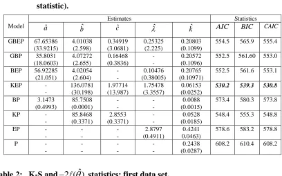
Table 1 lists the MLEs (the corresponding standard errors in parentheses) of the parameters of all the models for the first data set (the exceedances of flood peaks data) and the statistics: Akaike information criterion (AIC), Bayesian information criterion (BIC) and consistent Akaike information criterion (CAIC). Table 2 gives the values of the statistics Kolmogorov-Smirnov (K-S) and 2 ( )ˆ (where ( )ˆ denotes the
log-likelihood function evaluated at the maximum log-likelihood estimates) for the first data set. The results of the last four models (BP, KP, EP and P) can be obtained from Bourguignon et al. (2013). Since the KEP distribution has the lowest AIC, BIC, CAIC, 2 ( )ˆ and K-S values among all the other models, and so it could be chosen as the best model. Additionally, it is evident that the P distribution presents the worst fit to the first data.
Tables 3 and 4 provide the MLEs (the corresponding standard errors in parentheses) of the parameters of all the models and the statistics AIC, BIC, CAIC, 2 ( )ˆ and K-S for
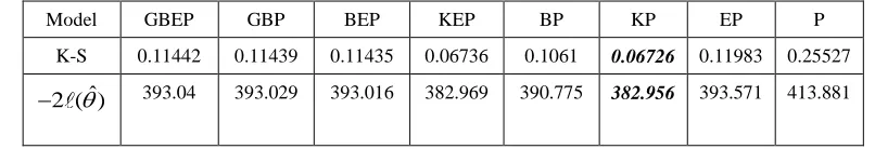
the second data set (actual taxes revenue). Again, the results indicate that the KP model presents the smallest values for the AIC, BIC, CAIC, 2 ( )ˆ and K-S statistics among
Table 1: MLEs (standard errors in parentheses) and the statistics AIC, BIC and CAIC; first data set. (ˆd 0.1 for all models, Sinceˆd is the first order statistic).
Model
Estimates Statistics
ˆ
a bˆ cˆ ˆ kˆ AIC BIC CAIC
GBEP 67.65386 (33.9215) 4.01038 (2.598) 0.34919 (3.0681) 0.25325 (2.225) 0.20803 (0.1099)
554.5 565.9 555.4
GBP 35.8031
(18.0603) 4.07272 (2.655) 0.16468 (0.3836) - - 0.20572 (0.1096)
552.5 561.60 553.0
BEP 56.92285
(21.051) 4.02054 (2.604) - - 0.10476 (0.38005) 0.20765 (0.10971)
552.5 561.6 553.1
KEP -
- 136.0781 (30.198) 1.97714 (13.987) 1.75478 (3.3557) 0.06153 (0.0252)
530.2 539.3 530.8
BP 3.1473
(0.4993) 85.7508 (0.0001) - - - - 0.0088 (0.0015)
573.4 580.3 573.8
KP -
- 85.8468 (0.3371) 2.8553 (0.3371) - - 0.0528 (0.0185)
548.4 555.3 548.8
EP -
- - - - - 2.8797 (0.4911) 0.4241 0.0463)
578.6 583.2 578.8
P -
- - - - - - - 0.2438 (0.0287)
608.2 610.4 608.2
Table 2: K-S and2 ( )ˆ statistics; first data set.
Model GBEP GBP BEP KEP BP KP EP P
K-S 0.15665 0.16028 0.15663 0.14314 0.1747 0.1700 0.1987 0.3324
ˆ 2 ( )
655.646 544.494 544.529 522.211 567.4 542.4 574.6 606.2
Table 3: MLEs (standard errors in parentheses) and the statistics AIC, BIC and CAIC; second data set. (ˆd 4.1 for all models, Sinceˆd is the first order statistic).
Model ˆ Estimates Statistics
a bˆ cˆ ˆ kˆ AIC BIC CAIC
GBEP 50.173
(10.683) 1.61244 (0.782) 0.27553 (2.0699) 0.20069 (1.508) 1.09171 (0.406)
403.04 413.427 404.172
GBP 34.7029
(25.352) 1.61671 (0.986) 0.07979 (0.578) - - 1.08948 (0.5589)
401.029 409.34 401.77
BEP 27.025
(15.333) 1.622 (1.031) - - 0.10229 (0.566) 1.08673 (0.58)
401.016 409.326 401.757
KEP -
- 75.33529 (39.223) 1.41497 (20.494) 1.46209 (21.177) 0.11359 (0.105)
390.97 399.28 391.71
BP 2.57098
(0.44668) 17.09134 (6.4901) - - - - 0.1373 (0.5001)
396.775 403.008 397.212
KP -
- 77.3103 (22.144) 2.06776 (0.2537) - - 0.11195 (0.1033)
388.956 395.188 389.392
EP -
- - - - - 2.54142 (0.4883) 1.58491 (0.205)
397.571 401.726 397.786
P -
- - - - - - - 0.95346 (0.1241)
Table 4: K-S and 2 ( )ˆ statistics; second data set
Model GBEP GBP BEP KEP BP KP EP P
K-S 0.11442 0.11439 0.11435 0.06736 0.1061 0.06726 0.11983 0.25527
ˆ 2 ( )
393.04 393.029 393.016 382.969 390.775 382.956 393.571 413.881
6. Conclusion
The new five-parameter model (Since the sixth parameter is the first order statistic) includes as special sub-models the Pareto, exponentiated Pareto (Gupta et al., 1998), beta Pareto (Akinsete et al., 2008), Kumaraswamy Pareto (Bourguignon et al., 2013), beta generalized Pareto (Nassar and Nada, 2011), beta exponentiated Pareto (Zea et al., 2012), Kumaraswamy exponentiated Pareto (Elbatal, 2013) and generalized beta Pareto (new) distributions. We provide a mathematical treatment of this distribution including analytical expressions for the moments, moment generating function, mean deviations, mean residual life, Lorenz, Bonferroni and Zenga curves, quantile function and Rényi entropy. The estimation of the model parameters is approached by maximum likelihood and the observed information matrix is derived. The usefulness of the new model is illustrated in two applications to real data using goodness-of-fit tests.
Acknowledgment
The author thanks the Editor and the Referees for their helpful remarks that improved the original manuscript.
References
1. Akinsete, A., Famoye, F. & Lee, C. (2008). The beta-Pareto distribution.
Statistics, 42, 547-563.
2. Alexander, C., Cordeiro, G. M., Ortega, E. M. M. & Sarabia, J. M. (2012). Generalized beta generated distributions. Computational Statistics and Data Analysis, 56, 1880-1897.
3. Alzaatreh, A., Famoye, F. & Lee, C. (2012). Gamma Pareto distribution and its applications. Journal of Modern Statistical Methods, 11, 78-95.
4. Bourguignon, M., Silva, R. B., Zea, L. M. & Cordeiro, G. M. (2013). The Kumaraswamy Pareto distribution. Journal of Statistical Theory and Applications
12, 129-144.
5. Burroughs, S. M. & Tebbens, S. F. (2001). Upper-truncated power law distributions. Fractals, 9, 209-222.
6. Choulakian, V. & Stephens, M.A. (2001). Goodness-of-fit for the generalized Pareto distribution. Technometrics, 43, 478-484.
8. Corderio, G.M., Hashimoto, E.H. & Ortega, E.M.M. (2014). The McDonald Weibull model. Statistics, 48, 256-278.
9. Cordeiro, G. M., Ortega, E. M. M. & Nadarajah, S. (2010). The Kumaraswamy Weibull distribution with application to failure data. Journal of the Franklin Institute, 347, 1399 -1429.
10. Cordeiro, G.M., Pescim, R.R. & Ortega, E.M.M. (2012). The Kumaraswamy generalized half-normal distribution for skewed positive data. Journal of Data Science, 10,195-224.
11. de Castro, M.A.R., Ortega, E.M.M. & Cordeiro, G.M. (2011). The Kumaraswamy generalized gamma distribution with application in survival analysis. Statistical Methodology, 8, 411- 433.
12. ElbataL (2013). The Kumaraswamy exponentiated Pareto distribution. Economic Quality Control, 28, 1-9.
13. Eugene, N., Lee, C. & Famoye, F. (2002). The beta-normal distribution and its applications. Communications in Statistics -Theory and Methods, 31, 497-512.
14. Famoye, F., Lee, C. & Olumolade, O. (2005). The beta-Weibull distribution.
Journal of Statistical Theory and Applications, 4, 121-136.
15. Gradshteyn, I. S. & Ryzhik, I. M. (2007). Table of integrals, series and products.
Seventh Edition, Alan Jeffrey and Daniel Zwillinger (eds.), Academic Press.
16. Gupta, R.C., Gupta, R.D. & Gupta, P.L. (1998). Modeling failure time data by Lehman alternatives. Communications in Statistics-Theory and Methods ,27, 887-904.
17. Jones, M.C. (2004). Families of distributions arising from distributions of order statistics. Test, 13, 1-43.
18. Kleiber, C. & Kotz, S. (2003). Statistical size distributions in economics and actuarial sciences. Wiley Series in Probability and Statistics. John Wiley & Sons.
19. Kong, L., Lee, C. & Sepanski, J.H. (2007). On the properties of beta-gamma distribution. Journal of Modern Applied Statistical Methods, 6, 187-211.
20. Kumaraswamy, P. (1980). Generalized probability density function for double bounded random processes. Journal of Hydrology, 462, 79-88.
21. Mahmoudi, E. (2011).The beta generalized Pareto distribution with application to lifetime data. Mathematics and Computers in Simulation, 81, 2414-2430.
22. Marciano, F.W.P., Nascimento, A.D.C., Santos-Neto, M. & Corderio, G. M. (2012). The Mc-distribution and its statistical properties: an application to reliability data. International Journal of Statistics and Probability, 1, 53-71.
23. Nadarajah, S. & Kotz, S. (2006). The beta exponential distribution. Reliability Engineering & System Safety, 91, 689-697.
24. Nassar, M. M. & Nada, N. K. (2011).The beta generalized Pareto distribution.
25. Oluyede, B. O. & Rajasooriya, S. (2013). The Mc-Dagum distribution and its statistical properties with applications. Asian Journal of Mathematics and Applications, 44, 1-16.
26. Schroeder, B., Damouras, S. & Gill, P. (2010). Understanding latent sector error and how to protect against them. ACM Transactions on Storage (TOS), 6(3), Article 8.
27. Tahir, M. H., Mansoor, M., Zubair, M. & Hamedani, G. G. (2014). McDonald log-logistic distribution with an application to breast cancer data. Journal of Statistical Theory and Applications, 13, 65-82.
28. Zea, L. M., Silva, R.B., Bourguignon, M., Santos, A., M. & Cordeiro, G. M. (2012). The beta exponentiated Pareto distribution with application to bladder cancer susceptibility. International Journal of Statistics and Probability, 2, 8 -19.