On the protein folding problem in 2D-triangular lattices

(1)

2D-triangular lattices

Abu Sayed Md Sohidull Islam and Mohammad Sohel Rahman

*

Abstract

In this paper, we present a novel approximation algorithm to solve the protein folding problem in HP model. Our algorithm is polynomial in terms of the length of the given HP string. The expected approximation ratio of our

algorithm is 1−2 logn

n−1 forn≥6, wheren

2_{is the total number of H’s in a given HP string. The expected approximation}

ratio tends to reach 1 for large values ofn. Hence our algorithm is expected to perform very well for larger HP strings.

Keywords: Protein folding, Approximation ratio, Algorithms, HP model

Background

A long standing problem in Molecular Biology and Bio-chemistry is to determine the three dimensional struc-ture of a protein given only the sequence of amino acid residues that compose protein chains. This problem is known as the Holy Grail of Computational Molecular Biology, also termed as “cracking the second half of the genetic code”. There exist a variety of models attempting to simplify the problem by abstracting only the “essential physical properties” of real proteins. In these models, the three-dimensional space is often represented by a lattice. Residues which are adjacent (i.e., covalently linked) in the primary sequence must be placed at adjacent points in the lattice.

In this paper, we consider the Hydrophobic-Polar Model, HP Model for short, introduced by Dill [1]. The HP model is based on the assumption that hydrophobic-ity is the dominant force in protein folding. This model simplifies a protein’s primary structure to a linear chain of beads. Each bead represents an amino acid, which can be one of two types: H (hydrophobic or nonpolar) or P (hydrophilic or polar). Conformations of proteins are embedded in either a two-dimensional or three-dimensional square/triangular/hexagonal lattice. A con-formationof a protein is simply a self-avoiding walk along the lattice. The goal of the protein folding problem is to

*Correspondence: [email protected]

AEDA Group, Department of CSE, BUET, Dhaka 1000, Bangladesh

find a conformation of the protein sequence on the lat-tice such that the overall energyis minimized, for some reasonable definition of energy. Each amino acid in the chain is represented by occupying one lattice point, con-nected to its chain neighbour(s) on adjacent lattice points. An optimal embedding is one that maximizes the num-ber of H-H contacts which are not adjacent in the amino acid chain. So, in effect, an input to the problem is a finite string over the alphabet(H,P)+. Often, in what follows, the input strings to our problem will be referred to as HP strings. For a more biological background and motivations the readers are referred to [1,2].

A number of approximation algorithms have been developed for the HP model on the 2D square lattice, 3D cubic lattice, triangular lattice and the face-cantered-cubic (FCC) lattice [3-5]. The first approximation algo-rithm developed for this problem on the square lattice by Hart and Istrail has an approximation ratio of 1/4 [3]. The approximation ratio for this problem was improved to 1/3 by Newman [4]. The algorithm presented in [3] can be generalized to an approximation algorithm for the problem on the 3D cubic lattice. In [6], a general method for protein folding on the HP model was pre-sented by Hart and Istrail. This method can be applied to a large class of lattice models. Hart and Istrail [7] provided the first approximation algorithn for the problem on the side-chain model which can be applied to 2D square, 3D cubic lattices, and FCC lattices. The approximation ratio achieved by [7] remains the best ratio for an approxima-tion algorithm in any 3D HP-models to date. In [7], the

(2)

Islam and RahmanAlgorithms for Molecular Biology2013,8:30 Page 2 of 14 http://www.almob.org/content/8/1/30

authors also illustrate the transformation of approxima-tion algorithm from lattice models to off-lattice models. Another approximation algorithm, based on different geo-metric ideas was presented in [5]. Heun [8] presented a linear-time approximation algorithm for protein folding in the HP side chain model on extended cubic lattice having approximate ration 0.84. In [9], the authors presented an approximation algorithm with approximation ratio 0.17 that folds an arbitrary protein sequence in the 2D hexag-onal lattice HP-model. Readers are referred to a survey of Istrail and Lam [10] for further reading.

In [11], the authors proposed a genetic algorithm for the protein folding problem in HP model in 2D square lat-tice. In [12,13], hybrid genetic algorithm was presented for HP model in 2D triangular lattice and 3D FCC lat-tice. The authors in [14] first proposed thepull move set

for rectangular lattices, which is used in the HP model under a variety of local search methods. They also showed the completeness and reversibility of the pull move set for rectangular grid lattices. In [15], the authors extended the idea ofpull move setin local-search approach for finding an optimal embedding in 2D triangular grid and the FCC lattice in 3D.

In this paper, we present an approximation algorithm for protein folding in 2D-triangular lattice. To the best of our knowledge the best approximation ratio for this problem was obtained by Agarwalla et al. [2], which is ₁₁6. For our algorithm we do a probabilistic analysis and deduce that the expected approximation ratio of our algorithm is 1−

2 logn

n−1 forn ≥ 6, wheren2is the total number of H in a

given HP string. Clearly our approximation ratio depends onn, which in turn depends on the number of H in the HP string. For large values ofn, this ratio tends to reach 1. So it can be expected that our algorithm would provide very close to optimal results for large values ofn.

The rest of the paper is organized as follows. In Section ‘Preliminaries’, we define some notations and notions. Section ‘Our approach’ describes our approach to solve the problem. In Section ‘Expected approximation ratio’ we deduce the expected approximation ratio. We briefly conclude in Section ‘Conclusion’.

Preliminaries

In this section, we present some notions and definitions (mostly in relation to the underlying lattice) that we need to explain our algorithm. In a triangular lattice, each lat-tice point has six neighbouring latlat-tice points [2]. In the literature it is also called a hexagonal lattice. Note that, by definition, a lattice is infinite. However, in what fol-lows, when we refer to a lattice we will refer to a finite part of it. This finite part of the lattice would essentially be a hexagon. We now define some notions related to a hexagon in the context of our approach. Note that a

hexagon is said to be perfect (or regular) if it has six equal sides and six equal angles. Throughout the paper, when we refer to a hexagon we assume that the opposite sides of it are parallel having the same length. Also, when we con-sider a non-regular hexagon we assume that the sides of it can be grouped into two groups based on their length. In particular, two of its sides (that are parallel to each other) have a particular length, saypand the other four sides have a different length, saym. Clearly, whenp=m, we have a regular hexagon. Following the above discussion, it would be useful to define the former couple of sides of the (non-regular) hexagon (i.e., that having a length ofpeach) as D-sides and the latter four sides (i.e., that having a length ofmeach) asQ-sides.

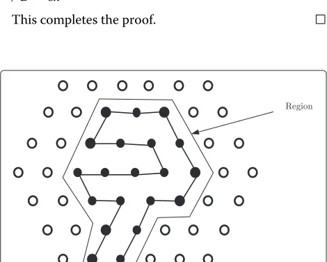
The discussion that follows can be better understood with the help of Figure 1. As has been mentioned above the finite portion of the lattice of our interest can be seen as a hexagon, theboundaryof which consists of those lat-tice points that have fewer than six neighbours within the hexagon. Anedge is formed by two neighbouring lattice points. If the lattice points are filled by H, the two neigh-bouring H’s also form an edge. If two H’s are non-adjacent in an HP string and placed on neighbouring lattice points to form an edge, they form a bond. The points on the boundary are referred to as the boundary points. The

depth of a point in a lattice is the minimum number of points it needs to traverse to reach any boundary point. Naturally, the depth of a boundary point is 0. The depth of a hexagon is the maximum depth of all points in the hexagon. In Figure 1, the depth of the hexagon is 2.

Thelengthof the hexagon (or lattice) is the total number of points along theD-sides. Figure 1, shows a hexagon of length 6. Aregionin the hexagon is a group of the lattice points such that each point in it has at least two neigh-bours from within it. Similar to the boundary of a hexagon we also define the boundary of a region. The boundary of a regionconsists of those lattice points that have fewer than six neighbours within the region. A region must not contain any point such that deleting that point creates two separate regions. From a graph theoretic concept, the region cannot have acut vertex. Also all the lattice points inside the boundary of a region are parts of the region. So, by definition, only the boundary itself cannot be con-sidered as a region unless there are no points inside the boundary at all. In Figure 1, the black vertices comprise a region (which has only one point inside the boundary). The size of a region is the total number of lattice points inside it including the boundary points.

(3)

Figure 1Lattice.In this figure, a lattice and some related notions are illustrated.

Figure 1. Notice that if the depth of such a hexagon isx, then a bend contains 2x+1 points. There is a total of

bends in a hexagon, whereis the length of the hexagon. Removing all bends from the hexagon leaves a total ofx2

lattice points (see Figure 1).

Now we define a new notion of a distorted hexagon as follows. Suppose we have a hexagon having lengthand depthx; so each bend contains 2x+1 points. Now we can increase its length to get a new hexagon of length+1 by adding a new bend. Similarly by adding succesive bends we can continue to increase the length of a hexagon. If within such a process the last added bend has fewer than 2x+1 points, then we refer to the hexagon as a distorted hexagon. An example of a distorted hexagon is shown in Figure 2.

We use the usual notion of arunin an HP string. In par-ticular, a run in an HP string denotes the consecutive H’s or P’s. For example, in the HP stringHHHPPHHPHHHH, we have a run of 3 H’s, followed by a run of 2 P’s and so on. Here therun-lengthof the first run of H (P) is 3 (2). We sometimes will use the term H-run (P-run) to indicate a run of H’s (P’s). The longest H-run (P-run) of a string denotes the run of H (P) which has the highest run-length among all the H-runs (P-runs) of the string. For the sake of conciseness, the HP strings shall often be represented as H’s and P’s with the corresponding run-lengths as their powers. So, the HP stringS = HHHPPHHPHHHH will often be conveniently represented bySˆ = H3P2H2P1H4. Further, we useS(i), 1≤i≤ |S|to denote theith charac-ter of the HP stringS. Similarly,Sˆ(j)denotes thejth run ofSˆ. For example,Sˆ(1)refers toH3_,_Sˆ₍₂₎_{refers to}_P2_and

so on. We will useSumHas the sum of the run-lengths of all the H-runs of a given stringSˆ. We end this section with a formal definition of the problem we handle in this paper.

Problem 1.Given an HP stringSˆ, the problem is to place the HP string on a triangular lattice such that the total number of bonds are maximized.

Our approach

Our approach is a simple and intuitive one. Our idea is to identify the length and depth of a suitable hexagon and then try to put all the H’s of a particular H-run inside the hexagon and put the P’s of the following P-run (if any) out-side that hexagon. The length and depth of the hexagon depend on SumH. The motivation here is to get the maxi-mum number of bonds between H’s. Note carefully that if we can fully fill a hexagon withzlattice points with a single H-run and get a total ofkedges, the number of total bonds will bek−z+1. And if the number of H-run isn(H)then in this case the total number of bonds will bek−z+n(H). We illustrate the approach with an example below. In the figures throughout this paper the bonds and edges are not shown explicitly. A connection between 2 lattice points indicate the presence of 2 H’s that are adjacent in the input HP string.

Example 1.Suppose we have an HP string as follows:

ˆ

S =H6P5H2P6H4P5H6P3H2P5H4PH7P6H2P2H4.

(4)

Figure 2Distorted hexagon.In this figure, a distorted hexagon is illustrated.

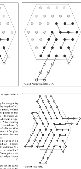
Figure 9. The final position of all the runs ofSˆis shown in Figure 10.

In Figure 10, we have a hexagon of 37 points and after filling the hexagon fully we get a total of 90 edges. It is easy to verify that the total number of bonds are 62 which is equal tok−z+n(H). Notably, if two hexagons have the same number of lattice points and are filled up fully with H by a given HP string, the hexagon with higher number of total edges have the higher number of total bonds as the difference between the total number of the edges and that of bonds is a constant.

Figure 3Lattice points, i.e., Hexagon.

Now that we have discussed our main approach to fill up the hexagon, we can shift our focus to the question of whether we can accommodate all the H-runs of the input HP string within the current hexagon. Recall that our goal is to increase the number of edges (and hence the total number of bonds)as much as possible. We have the following useful lemmas.

Lemma 1.If two hexagons have the same number of lat-tice points then the hexagon with the higher depth will not have lesser number of edges.

(5)

Figure 5Positioning_Sˆ(14)₌P6_.

Figure 6PositioningSˆ(15)=H2_.

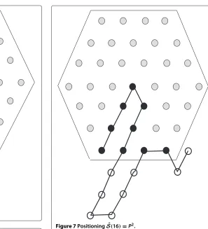
Figure 7Positioning_Sˆ(16)=P2_.

Proof.We show this by considering a hexagon and adjusting its depth keeping the total number of points fixed. We illustrate this scenario in Figure 11. Note that, the adjustment discussed and shown here does not give us a hexagon and is only to facilitate better exposition of the calculation and arguments.

Suppose that the total number of points isz and the depth of the hexagonxand length. If we remove the top and bottom rows and put the corresponding points along the other rows of the hexagon, new bends to the either side of the hexagon will be created and each bend will have 2×(x−1)+1 points. The new hexagon will have depth

x−1 and additional ₂_x2₋₁ ≥1 bends (see Figure 11). Now deleting two rows decrease 2× (2+−1)or 6−2 edges. On the other hand, increasing the₂_x2₋₁bends will increase ₂_x2₋₁×((2x−2)+(2x−1)+(2x−2))or

2

2x−1×(6x−5)or 2

2x−1×(3(2x−1)−2)or 6− 4 2x−1edges.

This is clearly less than or equal to 6−2 as₂_x4₋₁−2≥0 or₂_x2₋₁ ≥1. Hence the result follows.

(6)

Figure 8Positioning_Sˆ(13)=H4_.

as well. ThenH2will have lesser number of edges inside it than that ofH1.

Proof. Suppose that the depth of the regular hexagonH1

isx. So the length isx+1. To reduce the length ofH1,

while keeping the total number of points intact, we have to remove a bend ofH1and distribute the points on that

bend over the adjacent sides (See Figure 12). HenceH2

will be a non-regular hexagon. Note that a bend in a regu-lar hexagon contains 2x+1 lattice points. After reducing the length, new length will becomex−1 as follows. By deleting one bend we reduce the length of adjacent sides by one. So they will now havexlattices points. After plac-ing the removed lattice points over these sides the new side will definitely havex−1 lattice points.

Now deleting a bend decreases 2×2x+1+2xor 6x+1 edges. Out of the 2x+1 points of the bend, 2x−2 points will create new sides. These points create additional 2×

(2×(x−1)+x−2)or 6x−8 edges. And the rest of the 3 points can contribute to at most 8 edges. So we get at most a total of 6xedges whereas we loose 6x+1 edges. Hence the result follows.

Lemma 3. Assuming that we can fill up all the points of the hexagon, the total number of edges (as well as the

Figure 9PositioningSˆ(13)=H6.

(7)

Points to be deleted

New points forming bends

Figure 11Figure for Lemma 1.This figure aids in understanding the proof of Lemma 1.

total number of bonds) will be maximum if, and only if, the hexagon is a regular hexagon.

Proof.Lemma 3 follows readily from Lemmas 1 and 2.

As has been mentioned before, our algorithm proceeds in an iterative fashion in order to achieve the highest pos-sible number of edges by iteratively changing the length and depth of the hexagon. We start with an appropriate regular hexagon. Note carefully that, by Lemma 3, if we can fill the points of a regular hexagon, we get the opti-mum number of edges. If we fail to fill up all the points

of a regular hexagon we put the rest of the H-runs out-side the hexagon in a single row (see Figure 13) and finally compute the total number of bonds. We reduce the depth of the hexagon and increase its length with the hope that the number of bonds will increase in the new hexagon. We continue the iteration (i.e., reducing the depth of the hexagon and filling it up) until we reach a case when the total number of bonds decreases than that of the previ-ous iteration. In that case, we terminate our algorithm and return the result of the previous iteration.

Notably, to fill up a regular hexagon with depthxat least one H-run having length 2x+ 1 is needed. Besides, we need at least two H-runs of length 2x, three of length 2x−2,

(8)

Figure 13Sˆof Example 2 cannot properly fill the hexagon.This figure illustrates thatSˆof Example 2 cannot properly fill the hexagon.

three of length 2x−4. . .three H-runs of length 1 or 2 (depending on the size of x) in the input. The string in Example 1 presented before meets this criteria assuming

x = 3. To explain a bit more, note that, in the HP string of Example 1 we have one H-run with run-length 7, two H-runs with run-length 6, three H-runs with run length 4 and the rest of the H-runs have run-length 2. Another example is given below where we cannot put all H’s in a regular hexagon.

Example 2. Consider an HP string ˆ

S=H6P3H4P4H3P6H4P3H2P4H2P3H6P2H5P2H2PH3.

For this string, the length of a suitable regular hexagon is 4 (i.e., depth is 3) as SumH is 37. But in Figure 13 we can see that we cannot properly fill the hexagon. So we put the rest of the H-runs outside the hexagon in a single row. In such a case we have to increase the length of the hexagon to 6 as well as decreasing its depth to 2. The new hexagon is shown in Figure 14. It is evident from Figure 14, that we can now fill the hexagon properly withSˆand thus increase the total number of bonds.

Figure 14_Sˆof Example 2 can fill the adjusted hexagon.This figure illustrates thatSˆof Example 2 fill the adjusted hexagon.

Steps of the algorithm

Now we describe the steps of our algorithm below.

Step 1 Let SumH of the input HP stringSˆisz and the longest H-run isSˆ(i)having run-lengthk.

Computex= 1+

1+4×(z−1)

3

2 . SetglobalB=0. Step 2 Set= ₂z−_x₊x2₁and construct a hexagon with

lengthand depthx where each bend will contain2x+1points. Ifz≥(2x+1)+x2_then add newp bends such that

(+p)(2x+1)+x2_≥_z_≥₍₊_p₊₁₎₍₂_x₊₁₎₊_x2_. Ifz> (+p)(2x+1)+x2then create a distorted hexagon having the last bend (i.e., on the boundary of the hexagon) containing z−(+p)(2x+1)+x2points.

Step 3 For each of the H-runs and P-runs, starting from ˆ

S(i)and wrapping around the end (if applicable) execute the following steps. For an H-run, execute Step 3.a, Step 3.b and Step 3.c; for a P-run execute Step 3.d.

Step a [for H-runs] If the run length of the H-run is less than 3 then we take lattice points on the boundary of the hexagon. Otherwise, we try to find a region from the remaining

unoccupied points as follows. Here the total number of points in the region must be equal to the

(9)

Step i Take two points on the boundary of the hexagon. These are the first two points of the regionR.

Step ii Identify the

unoccupied points in the hexagon such that each of those has two neighbouring lattice points inR. Find the point having the highest depth among these points (breaking ties arbitrarily) and add this point toR. Thus we increase the sizeR(by one). Step iii If no such point is

found then go to Step 3.b.

Step iv If the size ofRis still less than the run length of the current H-run, go to Step 3.a.ii.

Step b [for H-runs]Fill up the lattice points of the identified region (R) with the H-run.

Step c [for H-runs]Put the rest of the H-runs (if any) outside the hexagon in a single row.

Step d [for P-runs]Put the P-run outside the hexagon in two rows. The first P of the run will be a neighbour of the previous H-run’s last H, while the last P of the run will be a neighbour of the next H-run’s first H.

Step 4 Count the total number of bonds,B. Step 5 IfglobalB>B, returnglobalB.

Step 6 Otherwise setglobalB=Bandx=x−1. Step 7 Ifx=1, returnB ; otherwise go to Step 2.

A brief discussion on Step 3.a.ii is in order. In Step 3.a.ii, our algorithm always chooses the points having the higher depths, with ties broken arbitralily. In some cases, some lattice points may remain unoccupied. Example 2 elabo-rates such cases. If some lattice points remain unoccupied

put the rest of the H-runs or parts thereof (as appropriate) outside the hexagon. The algorithm is formally presented in Algorithm 1.

Algorithm 1Finding the Folding

1: z←SumH ofSˆ

2: x← 1+

1+4×(₃z−1)

2

3: globalB←0

4: repeat

5: ← ₂z−_x₊x2₁

6: Findpsuch that(+p)(2x+1)+x2≥ z ≥(+ p+1)(2x+1)+x2

See Step 2 of Section ‘Steps of the algorithm’

7: Create a hexagonHwith length+pand depthx 8: ifz> (+p)(2x+1)+x2then

9: q←z−(+p)(2x+1)+x2

Determine the size of the bend having fewer than 2x+1 points

10: Add a bend withqpoints onH

Creates distorted hexagon

11: end if

12: foreach of the H-runs and P-runs, starting from

ˆ

S(i) and wrapping around the end (if applicable)

do

13: for H-runs follow Steps 3.a, 3.b and 3.c of Section ‘Steps of the algorithm’

14: for P-runs follow Step 3.d of Section ‘Steps of the algorithm’

15: end for

16: B←the total number of bonds inH 17: ifglobalB<Bthen

18: globalB←B

19: x←x−1 20: end if

21: untilglobalB≥Borx=1 22: return globalB

(10)

Figure 15Folding produced by Algorithm 1 with a hexagon havig depth 3 for_Sˆ1.This figure illustrates the folding produced by by Algorithm 1 ofSˆ1of Section ‘Steps of the algorithm’ for hexagon having depth 3.

reducing the depth by 1. The new folding produced in the next iteration is shown in Figure 17. Since the num-ber of bonds in this folding is less than that of Figure 15, Algorithm 1 will choose the folding of Figure 15. So, as expected, Algorithm 1 may not produce the optimal fold-ing for a hexagon with a given depth but it compares the folding produced by different hexagon having different depths and choose the best folding among there. As will be proved later, the folding produced by Algorithm 1 is expected to be quite near to optimal for long HP string. Now we present and prove the following theorem which basically proves the correctness of our approach.

Theorem 1. Given a region consisting of lattice points, a starting and an ending points such that those are boundary points of the hexagon, there always exists a path that starts at the starting point, ends at the ending point visiting each point in the region exactly once.

Figure 16Optimal folding for hexagon with depth 3 for_Sˆ1.This figure illustrates the optimal filling ofSˆ1of Section ‘Steps of the algorithm’ for hexagon having depth 3.

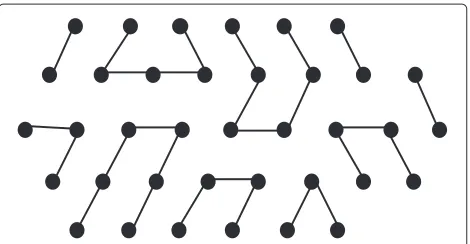
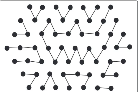
Proof. We can traverse the points row wise from left to right within the region starting from, say, Rowiand then right to left in Row i +1 and so on. If the number of rows are even, then, in this manner we can traverse all the points (see Figure 18). If it is odd then we traverse in a similar way except for the last two rows, where we simulta-neously traverse those in a zigzag fashion (see Figure 19). So filling up a region appropriately can be done in linear time with respect to the run-length of the corresponding H-run.

Our algorithm runs in polynomial time as discussed below. Firstly, the algorithm iterates over at mostxtimes. Now we havex≤√z, because,z=3×x×(x+1)which is proved in Lemma 4 in the following section. In each iter-ation we have to find a region for the current H-run. If a H-run has run-length, then Step 3.a in the algorithm needsO(2₎_{time as Step 3.a.ii needs at most}_O()_{time. So}

total time needed to perform this operation in each iter-ation, is at mostO(z2₎_{. As each of the other steps need}

constant time, the complete runtime of the algorithm is

O(z2×√z).

Expected approximation ratio

In this section, we are going to deduce the expected approximation ratio of our algorithm. As the total number of H-runs and run-lengths thereof may vary, in this anal-ysis, we will find the expected number of H-runs and the expected run-length of each of those. These two values will depend only on SumH. Consider a regular hexagon with depthx. Assume that the total number of points in the hexagon isz. Then we have the following lemma.

Lemma 4.Suppose we have a regular hexagon with depth x and z points. The total number of bonds, B, is6x2 when all the points are filled with H’s of a single H-run.

Proof. A regular hexagon with depth 1 have 1+6 = 7 points. We can increase its depth fromx−1 toxby adding 6xnew points each having depth 0. Since we havezpoints in the hexagon, so we must have:

z=1+6×1+6×2+6×3+. . .+6×x ⇒z=1+6×(1+2+3+. . .+x)

⇒z=1+6×(x+1)x/2

⇒z=1+3×x(x+1)

Now we will count the total number of possible edges,

(11)

Figure 17Folding produced by Algorithm 1 with a hexgaon having depth 2 for_Sˆ1.This figure illustrates the folding produced by by Algorithm 1 ofSˆof Section ‘Steps of the algorithm’ for hexagon having depth 2.

double counting, we have to divide the total count by two. So we have the following:

2×E=6×(3×x×(x+1)+1)−6×3−6×2

×(x−1)

⇒2×E=2×3×(3×x×(x+1)+1)−9+6−6x ⇒E=3×(3×x×(x+1)+1)−3−6x.

Now we focus on calculating the total number of bondsB. Recall that according to our approach, only H’s are placed inside the hexagon. Since an H can have at most 2 H’s adja-cent to it in an HP string, once placed inside the hexagon an H can only have at most 2 edges that would not be counted as bonds. So to computeB we simply need to deduct the total number of points fromE. So we have:

B=E−z+1

⇒B=3×(3×x(x+1)+1)−3−6x−(3×x(x+1) +1)+1

⇒B=2×(3×x(x+1)+1)−3−6x+1

⇒B=6×x(x+1)+2−3−6x+1

⇒B=6x2

This completes the proof.

Figure 18For even number of rows.This figure illustrates how to traverse all the points in a region with even number of rows.

Now the following lemma considers non-regular hexa-gons as well.

Lemma 5.Consider a hexagon (either regular or non regular) having n2points. Then, the total number of bonds B is less than or equal2×n(n−1).

Proof.According to lemma 4 for a regular hexagon with 1+3×x×(x+1)points, the total number of bonds is 6x2_{. Or replacing}_n₌_x₊_{1 we get, for a regular hexagon}

with 1+3×n×(n−1)points, the total number of bonds is 6×(n−1)2. So, clearly we have:

B≤n2×(6×(n−1)2)/(3×n(n−1)+1) ⇒B≤n2×(6×(n−1)2)/(3×n(n−1)) ⇒B≤2×n×(n−1)

Hence the result follows for regular hexagons. Clearly, by Lemma 3 the result applies for non-regular hexagons as well.

We will now deduce the approximation ratio based on an expected value of the total number of bonds. We assume that all H-runs have equal length. This assump-tion is valid in the context of our analysis and does not

(12)

lose generality as follows. In what follows, we will be work-ing with the expected number of H-runs and the expected length (saykEx) of an H-run. Hence in our analysis, each H-run will be assumed to have length kEx. We will now compute the expected values of the total number of edges (bonds),EEx(BEx) under this assumption.

From Figure 1, we can see that, the length of the hexagon isand depth isx. So each bend contains 2x+1 points and there are a total ofbends. There arex2remaining lattice points outside thebends. So if the total number of points arez(see Figure 1) then,

z=(2x+1)×+x2 (1)

So for a givenzandxwe can get,

= (z−x

2₎

2x+1 (2)

To calculate the total number of edges, at first we have to identify how many edges can be formed by individual points. The arguments of Lemma 4 for calculatingEand

Balso apply here. Note that, on the perimeter, aside from the corner points, total number of points are 2×(−2)+

4×(x−1). SoEExcan be computed as follows:

2EEx=6×((2x+1)×+x2)−6×3−2 ×(2×(−2)+4×(x−1)) ⇒2EEx=2×3×((2x+1)×+x2)−9

−(2−4+4x−4)

⇒EEx=3×((2x+1)×+x2)−1−2×(+2x)

AndBExcan be computed as follows:

BEx=EEx−z

BEx=3×((2x+1)×+x2)−1−2×(+2x) −((2x+1)×+x2)

⇒BEx=2×((2x+1)×+x2)−2×(+2x)−1

Hence, we get the following equation.

BEx=2z−2×(+2x)−1 (3)

Note that according to our approach, the value ofxis dependent on SumH. For this analysis, we now derive the expected run-length of H for a given HP string where SumH isn2. This problem can be mapped into the problem ofInteger Partitioningas defined below.

Problem 2. Given an integer Y, the problem of Integer Partitioning aims to provide all possible ways of writing Y, as a sum of positive integers.

Note that the ways that differ only in the order of their summands are considered to be the same partition.

A summand in a partition is called a part. Now, if we consider SumH as the input of Problem 2 (i.e., Y) then each run-length can be viewed as parts of the partition. So at first, we have to find the expected number of parti-tions, i.e., the expected number of runs of H. Kessler and Livingston [16] showed that to get an integer partition of an integerY, expected number of required parts is:

3Y

2π ×(logY+2γ −2 log

π

6),

whereγ is the famous Euler’s constant.

For our problemY =SumH=n2. If we denoteE[P] as the expected number of H-runs then,

E[P]=

6

π ×n×(logn+γ −log

π

6).

Now, as(logn+γ−log

π 6)≤(

2π

3 ×logn)forn≥5,

we can say that

E[P]≤2n×logn.

Since SumH is n2, expected value of each part, i.e., expected length of each run is greater than or equal to

n2

2n×logn = 2 logn n. Since all the H-runs are assumed to have the same length so each of them will construct a bend of 2x+1 points in the lattice. So we must have 2x+1≥ _{2 log}n _n. Hence we get the following equations:

x≥ n

4 logn−

1

2 (4)

≤

n2−(₁₆₍_logn2_n₎2 −_{4 log}n _n+1₄) n

2 logn

(5)

Now, let us consider a hexagonH1with lengthmax =

n2₋₍ n2

16(logn)2 − n

4 logn+

1 4)

n

2 logn

and depth xmin =

n

4 logn−

1

2. Now, inH1we also must haven

2_{points. So,}

from Lemma 1 and Equations 4 and 5, clearly the num-ber of bonds inH1is less than or equal to than that in the

hexagon having lengthand depthx. So from Equation 3 we have the following:

BEx≥2n2−2×(2nlogn−

n

8 logn−

logn

2n +

1 2

+ n

2 logn−1)−1

⇒BEx≥2n2−2×(2nlogn+ 3n

8 logn−

logn

(13)

BEx

B ≥

2n2−2×(2nlogn+

8 logn− 2n )

2n×(n−1)

⇒ BEx

B ≥

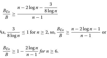
n−2 logn− 3

8 logn+

logn

2n2 n−1

As the termlogn

2n2 is very small we can ignore it from the

final result. Hence we have:

BEx

B ≥

n−2 logn− 3

8 logn n−1

As, 3

8 logn ≤1 forn≥2, so, BEx

B ≥

n−2 logn−1

n−1 or

BEx

B ≥1−

2 logn

n−1 for n≥6.

This is the final expected approximation ratio.

Note that the ratio increases significantly with the increase of the value ofnas presented in Table 1. So we can see that for large values ofn, expected approximation ratio tends to 1. So for largenit is expected that our algorithm will outperform the approximation algorithm presented in [2]. Recall that the approximation ratio of the algorithm of [2] is₁₁6, i.e., around 0.55.

Conclusion

In this paper, we have given a novel approximation algo-rithm to solve the protein folding problem in HP model introduced by Dill [1]. Our algorithm is polynomial and

the expected approximation ratio is 1− 2 logn

n−1 forn ≥

Table 1 Expected approximation ratio for different values ofn

logn n z=n2 _Ratio

3 8 64 0.142

4 16 256 0.466

5 32 1024 0.677

6 64 4096 0.809

This table illustrates the expected approximation ratio for different values ofn.

our algorithm is expected to perform very well for larger HP strings.

Competing interests

The authors declare that they have no competing interests.

Authors’ contributions

ASMSI proposed the algorithms. MSR verified the correctness of the algorithm and analysis. Both the authors read and approved the manuscript.

Acknowledgements

The authors would like to thank Md. Mahbubul Hasan for fruitful discussions. The authors gratefully acknowledge the fruitful comments and suggestions of the anonymous reviewers which aided in improving the presentation of the paper. This research work was conducted as part of the M.Sc. Engg. thesis work of Islam under the supervision of Rahman.

Received: 6 March 2013 Accepted: 20 November 2013 Published: 26 November 2013

References

1. Dill KA:Theory for the folding and stability of globular-proteins.

Biochemistry1985,24(6):1501–1509.

2. Agarwala R, Batzoglou S, Dancík V, Decatur SE, Hannenhalli S, Farach M, Muthukrishnan S, Skiena S:Local rules for protein folding on a triangular lattice and generalized hydrophobicity in the HP model.

J Comput Biol1997,4(3):275–296.

3. Hart WE, Istrail S:Fast protein folding in the hydrophobic-hydrophillic model within three-eights of optimal.J Comput Biol1996,3:53–96. 4. Newman A:A new algorithm for protein folding in the HP model.

In SODA ACM/SIAM2002:876–884.

5. Newman A, Ruhl M:Combinatorial problems on strings with applications to protein folding.InLATIN , Volume 2976 ofLecture Notes in Computer Science.Springer; 2004:369–378.

6. Hart WE, Istrail S:Invariant patterns in crystal lattices: implications for protein folding algorithms (Extended abstract).InCPM , Volume 1075 ofLecture Notes in Computer Science.Springer; 1996:288–303. 7. Hart WE, Istrail S:Lattice and off-lattice side chain models of protein

folding: linear time structure prediction better than 86% of optimal.

J Comput Biol1997,4(3):241–259.

8. Heun V:Approximate Protein Folding in the HP Side Chain Model on Extended Cubic Lattices.InLecture Notes in Computer Science 1643: Proceedings of the 7th Annual European Symposium on Algorithms.

Springer-Verlag; 1998:212–223.

9. Jiang M, Zhu B:Protein folding on the hexagonal lattice in the Hp model.J. Bioinformatics Computat Biol2005,3:19–34.

10. Istrail S, Lam F:Combinatorial algorithms for protein folding in lattice models: a survey of mathematical results.Commun Inf Syst2009,

9(4):303–346.

11. Unger R, Moult J:Genetic algorithms for protein folding simulations.

J Mol Biol1993,231:75–81.

12. Hoque T, Chetty M, Dooley LS:A hybrid genetic algorithm for 2D FCC hydrophobic-hydrophilic lattice model to predict protein folding.

InAustralian Conference on Artificial Intelligence, Volume 4304 ofLecture Notes in Computer Science.Springer; 2006:867–876.

13. Hoque T, Chetty M, Sattar A:Protein folding prediction in 3D FCC HP lattice model using genetic algorithm.InIEEE Congress on Evolutionary Computation.IEEE; 2007:4138–4145.

(14)

Conference on Research in Computational Molecular Biology (RECOMB) 2003.

ACM Press; 2003:188–195.

15. Böckenhauer HJ, Ullah AZMD, Kapsokalivas L, Steinhöfel K:A local move set for protein folding in triangular lattice models.InWABI, Volume 5251 ofLecture Notes in Computer Science.Springer; 2008:369–381. 16. Kessler I, Livingston M:The expected number of parts in a partition

of n.Monatshefte für Mathematik1976,81(3):203–212.

doi:10.1186/1748-7188-8-30

Cite this article as:Islam and Rahman:On the protein folding problem in 2D-triangular lattices.Algorithms for Molecular Biology20138:30.

Submit your next manuscript to BioMed Central and take full advantage of:

• Convenient online submission

• Thorough peer review

• No space constraints or color ﬁgure charges

• Immediate publication on acceptance

• Inclusion in PubMed, CAS, Scopus and Google Scholar

• Research which is freely available for redistribution