Spatial and temporal variability of snow depth and ablation rates in a small mountain catchment

(1)

www.the-cryosphere.net/4/215/2010/ doi:10.5194/tc-4-215-2010

The Cryosphere

Spatial and temporal variability of snow depth and ablation rates in

a small mountain catchment

T. Gr ¨unewald, M. Schirmer, R. Mott, and M. Lehning

WSL Institute for Snow and Avalanche Research SLF, 7260 Davos Dorf, Switzerland Received: 22 December 2009 – Published in The Cryosphere Discuss.: 13 January 2010 Revised: 2 May 2010 – Accepted: 10 May 2010 – Published: 28 May 2010

Abstract. The spatio-temporal variability of the mountain snow cover determines the avalanche danger, snow water storage, permafrost distribution and the local distribution of fauna and flora. Using a new type of terrestrial laser scan-ner, which is particularly suited for measurements of snow covered surfaces, snow depth was monitored in a high alpine catchment during an ablation period. From these measure-ments snow water equivalents and ablation rates were calcu-lated. This allowed us for the first time to obtain a high res-olution (2.5 m cell size) picture of spatial variability of the snow cover and its temporal development. A very high vari-ability of the snow cover with snow depths between 0–9 m at the end of the accumulation season was observed. This vari-ability decreased during the ablation phase, while the domi-nant snow deposition features remained intact. The average daily ablation rate was between 15 mm/d snow water equiv-alent at the beginning of the ablation period and 30 mm/d at the end. The spatial variation of ablation rates increased dur-ing the ablation season and could not be explained in a sim-ple manner by geographical or meteorological parameters, which suggests significant lateral energy fluxes contributing to observed melt. It is qualitatively shown that the effect of the lateral energy transport must increase as the fraction of snow free surfaces increases during the ablation period.

1 Introduction

The largest part of annual winter precipitation in the Alps above 1000 m a.s.l. falls as snow. Most of this precipitation is stored in the snow cover until melting starts at the end of the accumulation season. The amount and timing of the melt strongly depend on the thickness and the spatial distribution

Correspondence to: T. Gr¨unewald ([email protected])

of the snow cover. Hence the spatial and temporal variabil-ity of the snow cover greatly impacts the alpine water bal-ance and strongly affects nature and mankind (Elder et al., 1998). Drinking water supplies, hydro-power, agriculture and vegetation growth, all strongly depend on snow cover and alpine water storage (Keller et al., 2000; Jones et al., 2001; Armstrong and Brown, 2008). Moreover rapid melt-ing can cause floodmelt-ing and increased erosion (e.g. Male and Gray, 1981; Pomeroy and Gray, 1995). Furthermore, winter tourism, with its high economic importance in many alpine regions, strongly depends on snow reliability and snow cover duration (e.g. Haefner et al., 1997; Beniston, 2000; Fazzini et al., 2004; L´opez-Moreno and Nogu´es-Bravo, 2006; Marty, 2008).

To make reliable assessments of current and future snow dynamics, it is essential to obtain a better understanding of the total amount of snow stored in a catchment and how snow cover changes in space and time, especially in the ablation period.

(2)

LiDAR altimetry is a promising method to obtain area-wide high resolution snow depth data. Airborne laser scan-ning (ALS) proved to be an appropriate and accurate method for gathering area-wide snow depth measurements (Hopkin-son et al., 2001; Deems and Painter, 2006). ALS data were used to investigate spatial variability and scale invariance of snow depth and its relationship to wind direction, vegetation and topography for several mountainous test sites (Deems et al. 2006; Trujillo et al. 2007).

In recent years, the introduction of terrestrial laser scan-ning (TLS) to snow science has given a further push forward as this technology provides the possibility to obtain more cost effective and flexible area-wide snow depth observations with high spatial resolution (Bauer and Paar, 2004; J¨org et al., 2006; Prokop, 2008). Prokop et al. (2008) and Schaffhauser et al. (2008) performed detailed investigations on the accu-racy of TLS for measuring snow depth and showed that TLS is an appropriate tool for mapping snow depth with high ac-curacy.

However, so far this promising technique has not been used to focus on snow depth distributions and their time development for a catchment. By performing repeated TLS measurement campaigns in the Albertibach-catchment (Davos, Switzerland) during the entire ablation season of winter 2007/08, we present a unique data set of snow depth and SWE variability in a high mountain setting. The repeated catchment-wide measurement campaigns offer the possibil-ity to investigate seasonal snow cover changes by investigat-ing snow depth changes (mostly depletion) durinvestigat-ing the abla-tion phase.

This paper presents a first qualitative and quantitative in-vestigation of this dataset. We first give an overview of the study site and the methods used for collecting, processing and analysing the data. Then the spatial and temporal devel-opment of snow depth and SWE are analysed, followed by a detailed description of the ablation rates and an investigation of statistical correlations with weather and terrain parame-ters. Finally, conclusions of the main results of the study and a short outlook on future tasks and challenges are presented.

2 Method and data

2.1 Site description

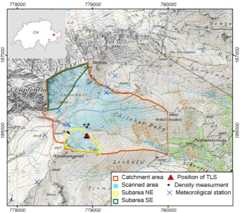
The area of investigation is a small mountain catchment lo-cated in the region of Davos, Switzerland (Fig. 1). The area of interest is defined by the drainage area of the Albertibach, which discharges in an easterly direction and is surrounded by steep mountain ridges to the north and south. The ele-vation of the area ranges from 1940 to 2658 m a.s.l. and is located above the local tree line. The total size of the catch-ment area is 1.3 km2, of which we covered 0.6 km2 (46%) in the laser surveys. The scanned area can be regarded as representative for the entire catchment in terms of elevation

Fig. 1. Location of the Albertibach catchment (marked with the

red line), the sub-areas NE (yellow line) and SE (green line), the area scanned in the TLS surveys (blue), the position of the TLS (red triangle) and of the meteorological stations in the area (blue crosses). Black stars indicate the position of the density samples taken at 26 April 2008. (base map: Pixelkarte PK25 © 2009 swis-stopo (dv033492))

range, aspect, and slope. The site is well equipped with a dense network of seven meteorological stations, which pro-vide continuous meteorological data.

3 Measurement methodology and accuracy assessment

We carried out four measuring campaigns to collect the data used in this study during the winter 2007/08. Surveys were made at the end of the accumulation season (26 April 2008) and at intervals of about two weeks until the end of the melt-ing season (13 May, 2 June and 10 June). The end of the ac-cumulation season was estimated from snow depth measure-ments at the permanent weather stations in the catchment.

(3)

position of the instrument was re-determined after each scan. Detailed information how to measure snow depth with TLS can be found in Prokop (2008).

We subjected all laser data to a variety of quality checks. In particular, we compared the laser measurements with those obtained from a tachymeter, as described in Prokop et al. (2008). With a tachymeter (Leica TCRP1201 total station) more than 500 single distance measurements were obtained on each of the four measurement campaigns. The tachymeter provided a very high accuracy for distance mea-surements at mid-range distances (up to 300 m) and there-fore provided an adequate method for the quality assessment (Prokop et al., 2008). The quality control revealed that snow depths showed mean deviations in the z-direction of less than 4 cm and standard deviations of less than 5 cm for distances of up to 250 m. This is a higher level of accuracy than that published by Prokop et al. (2008) and more than sufficient for our purposes.

Furthermore, an airborne laser scan is available for the end of the accumulation season using an independent helicopter based technology (Vallet et al., 2005; Skaloud et al., 2006). With this data, it was possible to investigate whether there were systematic errors in the terrestrial scans. The analysis showed that the ALS data had a mean deviation of less than 5 cm compared to a simultaneously performed tachymeter survey. The standard deviation was 6 cm. The spatial dis-tribution of the deviation in z-direction between the ALS and the TLS survey for 26 April is shown in Fig. 2. Comparing TLS and ALS gave a mean deviation of 10 cm and a standard deviation of 13 cm. The difference between TLS and ALS in-creased with the distance measured by the TLS as clearly vis-ible in Fig. 2 (blue colours). This is likely due to a decrease in accuracy of the TLS over long distances as the footprint of the laser beam increases. Furthermore, small deviations from the accurate position of the scanner’s origin have a larger in-fluence at larger distances. Especially in the areas with big differences between ALS and TLS, angles of incidence were worse for the TLS, which again affects the accuracy of the scan. The positive deviations (yellow and red areas in the east of the investigation area) were probably caused by a marginal movement or settling of the tripod, which caused a slight disposal of the TLS in comparison to the ALS for that area. Nevertheless the accuracy of the TLS is still more than sufficient for the analysis presented here.

3.1 Data processing

TLS measures the point distances from the scanner to the sur-face of the targets (snow sursur-face) with high spatial resolution and accuracy. To get absolute snow depths, the scans must be subtracted from a digital elevation model (DEM). The DEM used in this study was created from a summer TLS survey us-ing the same technology. A cell-size of 2.5 m was chosen for the DEM and for the resulting snow depth maps.

Fig. 2. Spatial distribution of the deviation in z-direction [m]

be-tween ALS and TLS survey for 26 April 2008.

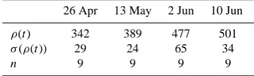
To calculate SWE and ablation rates from snow depth data, average snow cover density estimations are necessary. Many studies have found that the spatial variability of density is relatively small in comparison to snow depth (e.g. Dickin-son and Whiteley, 1972; Pomeroy and Gray, 1995; Marc-hand and Killingtveit, 2004; Mizukami and Perica, 2008). Consequently, it is common to estimate areal SWE with a small number of representative density measurements and a high number of snow depth data (e.g. Rovansek et al., 1993; Elder et al., 1998; Jonas et al., 2009). Thus, we calculated SWE based on a small number of well selected density mea-surements. Depth-average snow density is often assumed to be controlled by a small number of topographical and me-teorological parameters which are total snow depth, eleva-tion, solar radiaeleva-tion, climatic region and vegetation patterns (e.g. Anderton et al., 2004; Jonas et al., 2009). Because of the limited extent of the investigation area, we only focus on snow depth and solar radiation in this study.

(4)

Table 1. Depth-averaged snow density valuesρ(t) kg

m3 for each time

step, standard deviationσ(ρ(t)) and number of samples (n).

26 Apr 13 May 2 Jun 10 Jun

ρ(t) 342 389 477 501

σ(ρ(t)) 29 24 65 34

n 9 9 9 9

significant differences for the specific time steps (t )but no significant dependency on radiation classes R(t). We also investigated if a direct relationship between HS andρ(t) was obvious from the measurements but no general trend could be found. We hence decided to use a singleρ(t) for each time step which translates snow depth to SWE:

SW E=ρ(t )H S (1)

where SWE is in mm and HS in m. A summary of the calcu-latedρ(t )values is given in Table 1.

As a next step, we produced maps with the total SWE ap-plying Eq. 1 to each of the four snow depth maps. Maps of the average daily “ablation rate” were created by calculating daily ablation rates from the change between two consecutive SWE maps. The so called ablation rate can include contribu-tions from snow falls, settling, snow transport, snow subli-mation and true melting. As the SWE maps are the results of a simple linear relationship as given in Eq. (1), the patterns of the snow depth maps and the SWE maps are identical for each single time step. Hence we will focus our analysis on snow depth maps only and give the values for SWE in brack-ets where appropriate. Sinceρ is time dependent, the abla-tion rate and snow depth change maps did not show exactly the same patterns. But as there were no relevant differences in the characteristic features we focus on the results obtained from the daily ablation rates in what follows.

To refine the analysis, we separated two sub-areas from the investigation area (Fig. 1) based on the visual impression that two different snow distribution patterns may dominate these two sub-areas (Fig. 3): The first covers the north-easterly ex-posed slopes of Wannengrat, and will be referred to as NE in the following. It is characterized by a highly variable snow deposition on a rather large scale. The second sub-area con-sists of the southeast-facing slopes of the Vordere Latsch¨uel (SE), which appears to have a rather homogeneous snow dis-tribution.

3.2 Data analysis

A quantitative analysis of the raster maps allowed a de-tailed evaluation of the spatial and temporal variability of snow depth and the average ablation rates. We first visually interpreted the maps to identify obvious surface structures and characteristics. To quantify the spatial variability and

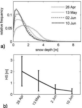
changes in time, histogram plots for the distribution of snow depth (Figs. 5a, 6) and the average ablation rates (Fig. 9) be-tween the individual scans were examined. Furthermore, we investigated basic statistics such as mean (µ), standard de-viation (σ) and total snow volume for each time period. For snow depthµandσalways refer to the area of the first survey (26 April), which is marked as “Scanned area” in Fig. 1. The histograms refer to the snow covered area of the respective survey.

For the daily ablation rates we only considered cells which still were snow covered on the second of two succeeding sur-veys. The snow covered area was determined with orthopho-tos, which were taken from a camera, which is an integral part of the TLS measurement set-up. We then focused on possible statistical dependencies of the ablation rate in the investigation area on topographic and meteorological param-eters. For this purpose, the Pearson’s linear correlation coef-ficient for the ablation rate as dependent variable was calcu-lated (Fig. 10). As independent variables we used:

– Topographical parameters derived from the DEM: alti-tude, slope, northing (difference in degrees from north). – Mean daily sum of incoming solar radiation, simulated with the physical based model Alpine3D (Lehning et al., 2006; Helbig et al., 2009), for each period of two suc-ceeding surveys. As input data for the model, we used data derived from an automatic weather and snow sta-tion located in the catchment. The model then produced hourly output for incoming shortwave radiation for each grid-cell of a 10 m-raster. We then averaged the output to one mean radiation day for each of the three periods. – SWE at the end of the accumulation season (SWEmax) derived from the TLS survey. The ablation rate as calcu-lated here contains also the contribution of settling and we therefore also investigated whether a correlation be-tween maximum snow depth or SWE and ablation rate exists.

(5)

Fig. 3. Snow depth maps for 26 April (a), 13 May (b), 2 June (c) and 10 June (d). The black arrows mark examples for snow filled ditches

To account for possible interactions between these param-eters, we combined the variables in multiple linear regres-sion models allowing for interaction terms. Only the models which performed best will be shown in the following.

4 Results and discussion

4.1 Time development of snow depth distribution

A map of the spatial snow depth distribution in the investiga-tion area for the end of the accumulainvestiga-tion season (26 April) is shown in Fig. 3a. The corresponding calculated SWE map is shown in Fig. 4. At that point in time, the entire catchment was snow covered, with exception of small snow-free patches

(6)

swisstopo (dv033492)).

Fig. 5. (a) Histograms and statistics (b) of snow depth (HS) at the

time of each scan. Only cells which were snow covered at the time of each scan are included to (a). Intervalsize 63. Statistics in (b) refer to the scanned area. The black line indicates the mean values and the error-bars the standard deviations.

Fig. 6. Histograms of snow depth for the sub-areas NE (a) and SE (b). Interval size for (a): 63, interval size for (b): 53.

The following scan, 17 days later, showed predominantly unchanged spatial patterns (Fig. 3b): The cornice- like drifts in the NE remained the dominant feature until the end of the ablation season while snow depth in the SE suffered stronger decrease than average (Fig. 3c, d; see also Fig. 6). A sig-nificant number of snow-free patches emerged especially on the knolls and ridges where snow depth was lowest in the beginning of the ablation season. Complete melt out prop-agated quickly from those first snow-free areas. This may be because of lower snow depths at the edges of the snow patches or because of lateral advective transport of heat from the warmer snow-free surfaces onto the colder snow cover (Essery and Pomeroy, 2004), which will be discussed in de-tail below.

Histograms of snow depth at the time of each scan show that the distribution and the variability changed in the course of the ablation season (Fig. 5a). The mean snow depth and the spatial variability, represented by the standard deviation (σ), both continuously decreased butσ remained on a high level (Fig. 5b). More interestingly, the standard deviation of snow depth still decreased when calculated for the snow covered area only. In fact, the numerical value was almost identical to the one based on the total area with deviations less than 10%.

(7)

There were clear differences in snow depth distribution between the two sub-areas SE and NE (Fig. 6a, b). The cornice-like drifts (discussed above), which featured the ar-eas maximum snow depth, were located in NE. The mean snow depths with 3.1 m (SWE = 1059 mm) were therefore larger in the NE than in the SE with 2.7 m (SWE = 919 mm) at the end of the accumulation season. A higher variability was also observed in the NE (σ = 1.7 m/569 mm) than in the SE (σ = 1.0 m/355 mm). This finding is also obvious from Fig. 3, where the more homogenous snow depth values in the SE are clearly visible. The context of higher variability and higher mean snow depth in the NE remained during the entire ablation season.

4.2 Spatio-temporal variability of ablation rates and their correlation with simple weather and terrain parameters

Ablation rates (as SWE) are shown in Fig. 7 and the cor-responding histograms are illustrated in Fig. 9 for all three investigation periods. For comparison, a map showing dif-ferences in snow depth is presented in Fig. 8. For the pe-riod from 26 April to 13 May the spatial differences in ab-lation rates with the highest rates in the steep south facing slopes and the lowest rates in the northern exposed slopes are clearly visible in Fig. 7a and represent the distribu-tion of potential radiadistribu-tion. The average abladistribu-tion rate was 15 mm/d (σ = 7 mm/d) for this period, increasing to 16 mm/d (σ= 7 mm/d) for the second and 30 mm/d (σ = 12 mm/d) for the last period (Fig. 9). This increase can easily be explained by the larger amount of energy, in the form of incoming solar radiation, available for melting later in the hydrological sea-son. It has to be noticed that no distinct change occurred between the first and the second period due to cool and moist weather during the second period. However, bothµ andσ strongly increased in the last period. While the spatial vari-ability of snow depth decreased (Figs. 3 and 5), the spatial variability of the ablation rates increased with time (Figs. 7 and 9).

Similar to the study of Anderton et al. (2004), we could only identify weak correlations between ablation rates and relevant topographic and meteorological parameters. Pear-son’s linear correlation coefficients are shown in Fig. 10 for all parameters and each time interval: Altitude, slope, nor-thing (each r=0.4), solar radiation (r=0.3) and wind-speedSE (r=0.3) provided the best correlations for the first period (26 April–13 May).

Note that the high correlation with slope, meaning that flat areas are characterised by smaller ablation rates, cannot be explained by relocation of snow from steep to flat areas due to avalanches, as no avalanches occurred during the ablation season.

For the second period (13 May –2 June) all high corre-lations from the first period decreased (slope: r=0.2, al-titude, northing each r=0.1, radiation r= −0.1,

wind-speedSE = 0.2) whereas SWEmax gave the best correlation withr= −0.4. In the final period (2 June–10 June) all corre-lations became very weak. This finding with the better cor-relations resulting from different parameters in comparison to period one, again suggests that the factors which dominate melt change in time. The strong decrease of the correlation is in this context attributed to the rising heterogeneity of the surface and of its energy balance which we already described above. The later in the ablation season, the smaller the direct influence of the parameters and the more “random” the abla-tion pattern appears. It is important to note that the ablaabla-tion pattern is not really random but determined by the distribu-tion of snow free patches in the vicinity, which is not rep-resented in local correlations. A further surprising outcome is the decrease of the correlation coefficient for windspeedSE although a major foehn event occurred in the second period. Local high windspeeds promote turbulent fluxes and there-fore affect the local energy balance. But advective effects as discussed below would not show up in such a local analysis and require a more involved analysis, which we plan to carry out in future.

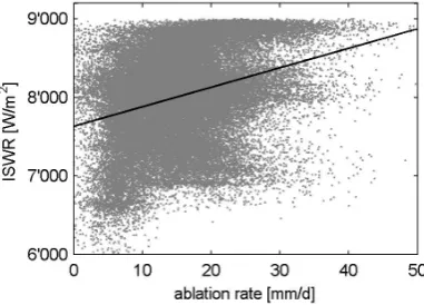
The weak correlations become even clearer when analysing the scatterplots of the ablation rates against the pre-dicting parameters. A scatter plot of ablation rates against incoming solar radiation is shown in Fig. 11. The large scat-tering of the data clearly illustrates that high statistical corre-lations cannot be expected from these data.

These findings lead to the conclusion that none of the sim-ple univariate parameters was adequate to explain spatial ab-lation characteristics to a satisfactory degree. A possible ad-ditional factor other than lateral energy transport discussed below may be that the spatial resolution of 2.5 m may still be too coarse. Windspeed was modelled on a spatial resolution of 5 m. A smaller horizontal resolution would strongly in-fluence the local windspeed distribution (Mott and Lehning, 2010). Patterns which were caused by the micro-relief are not captured by that resolution. Furthermore, there may be differences between the modelled meteorological variables and the true distribution, e.g. incoming radiation neglects fre-quent convective clouds over mountain tops.

(8)

Fig. 7. Daily ablation rates (SWE) averaged for the time periods 26 April–13 May (a), 13 May–2 June (b) and 2 June–10 June (c). (base

rat e1=4.2·alt it ude+7.6·slope+5.6·nort hing (2)

+3.8·radiat ion+12.2

For the second period anR2 of 0.3 was obtained from the model described in Eq. 3. Most variables which performed best in linear correlation analysis were also showing up in the multiple regression models, but in slightly different order. Slope was the most important variable in Eq. 2 and SWEmax accounted for the highest coefficient in Eq. 3.

rat e2= −2.1·alt it ude−8.8·slope−13.6·SW Emax (3)

+7.9·windspeed_NW+18.2

The last period did not give significant correlations. As has already been seen in the univariate correlations, we could

ob-serve a decrease in correlation with time and this was con-firmed by the multiple regressions. Therefore, the influence of topography and meteorology on ablation rates gets con-sistently weaker later in the ablation season. Using f-test, all regressions were found to be highly significant (p <0.001) which is not surprising when taking the large size of the sam-ple (N>18 000) into account.

(9)

Fig. 8. Daily ablation rate in snow depth (HS) averaged for the time

Fig. 9. Histograms of daily ablation rate (SWE). Interval size: 124.

shortwave radiation (r=0.3) described above. Later in the hydrological season the rapidly increasing fraction of snow free areas leads to changes in the energy balance: The sur-face albedo of snow free patches is small and causes higher surface temperatures and higher values of lateral sensible heat fluxes and longwave radiation, which then lead to in-creased melting of the surrounding snow patches (Essery and Pomeroy, 2004) especially at the edges of the patches. Thus, big differences in melting between small and larger snow patches may occur. Nonetheless, a comparison of coeffi-cient of variation values (CV=σ/µ) showed that the spatial variability of the ablation rates with CV – values of 0.4–0.5 was lower than the spatial variability of snow depth and SWE

Fig. 10. Coefficient of correlation (Pearson) for daily ablation rates for each time period against altitude, slope, northing, SWE at the end of the accumulation season (SWEmax), incoming short-wave radiation for each period (ISWR) and windspeed for prevailing wind direction north-west (windspeedNW)and south-west

(wind-speed_SW).

Fig. 11. Scatterplot of SWE ablation rates (26 April–13 May) and

mean daily sum of incoming shortwave radiation (ISWR). The solid line draws the linear fit function derived from the univariate regres-sion analysis.

(10)

melt season. Their results based on manual surveys are now confirmed by our more detailed dataset.

5 Conclusions

First results from an extensive data set on the spatio-temporal variability of snow depth were presented. The main focus of the analysis was on snow depth distribution but values for SWE were given where appropriate. We also present maps of the temporal changes of SWE, which are named “ablation rate” maps, although they are strictly the sum of real melt, sublimation and occasional smaller snowfalls.

Quality checks of the TLS measurement system against in-dependent tachymeter and ALS measurements showed good accuracy of the snow depth measurements such that the anal-ysis presented appeared not to be limited by measurement problems.

The results showed that spatial distribution and the vari-ability of snow depth remained similar for the whole abla-tion season. A striking result from the analysis of SWE de-velopment during the ablation phase is that a very variable distribution of ablation rates was observed. We conclude that advective transport of melt energy from snow free areas to re-maining snow patches was a major source for this variability and led to accelerated melt in the course of the ablation pe-riod in agreement with earlier results, which have been based on theoretical considerations (Essery and Pomeroy, 2004). This conclusion is consistent with the observation that ini-tial weak correlations of ablation rates with obvious meteo-rological and local terrain parameters became even weaker towards the end of the ablation period.

Beyond the first analysis presented here, the data set al-lows significant further and more in depth work, which we are currently undertaking. A major effort is devoted to a more quantitative understanding of lateral energy transport discussed above by using a combination of a meteorologi-cal with a detailed surface process model (ARPS/Alpine3D). The most direct application is an assessment of total snow water storage as compared to interpolations made from flat field snow stations (e.g. Bocchiola et al., 2008; Janetti et al. 2008) and the validation of snow deposition and snow trans-port models (Lehning et al., 2008). A further interesting as-pect is the development of surface roughness as a function of the variable snow cover.

Acknowledgements. We thank all people who helped during the ex-tensive field work and in data processing. Part of the work has been funded by the Swiss National Science Foundation and the European Community. This work would not have been possible without all colleagues from SLF who contributed to this work in various ways. For proofreading special thanks go to Alec van Herwijnen. We finally thank our three reviewers, Ruzica Dadic, Juraj Parajka and Davide Bavera for their constructive comments and corrections.

Edited by: D. Hall

References

Anderton, S. P., White, S. M., and Alvera, B.: Evaluation of spatial variability in snow water equivalent for a high mountain catch-ment, Hydrol. Process., 18, 435–453, 2004.

Armstrong, R. L. and Brown, R.: Introduction, in: Snow and Cli-mate, edited by: Armstrong, R. L. and Brun, E., Cambridge Uni-versity Press, Cambridge, 1–11, 2008.

Balk, B. and Elder, K.: Combining binary decision tree and geo-statistical methods to estimate snow distribution in a mountain watershed, Water Resour. Res., 36, 13–26, 2000.

Bauer, A. and Paar, G.: Monitoring von Schneeh¨ohen mittels ter-restrischem Laserscanner zur Risikoanalyse von Lawinen, 14th International Course on Engineering Surveying, Z¨urich, 15– 19 March 2004, 2004.

Bavera, D. and De Michele, C.: Snow water equivalent estimation in the Mallero basin using snow gauge data and MODIS im-ages and fieldwork validation, Hydrol. Process., 23, 1961–1972, doi:10.1002/hyp.7328, 2009.

Beniston, M.: Environmental Change in Mountains and Uplands, London UK and Oxford University Press, New York, 172 p., 2000.

Bl¨oschl, G.: Scaling issues in snow hydrology, Hydrol. Process., 13, 2149–2175, 1999.

Chang, K. T. and Li, Z.: Modelling snow accumulation with a geo-graphic information system, Int. J. Geogr. Inf. Sci., 14, 693–707, 2000.

Bocchiola, D., Bianchi Janetti, E., Gorni, E., Marty, C., and Sovilla, B.: Regional evaluation of three day snow depth for avalanche hazard mapping in Switzerland, Nat. Hazards Earth Syst. Sci., 8, 685–705, doi:10.5194/nhess-8-685-2008, 2008.

Dadic, R., Mott, R., Lehning, M., and Burlando, P.: Wind Influence on Snow Depth Distribution and Accumulation over Glaciers, J. Geophys. Res., 115, F01012, doi:10.1029/2009jf001261, 2010. Deems, J. S., Fassnacht, S. R., and Elder, K. J. Fractal Distribution

of Snow Depth from Lidar Data, J. Hydromet., 7, 285–297, 2006. Deems, J. S. and Painter, T. H.: Lidar measurement of snow depth: Accuracy and error sources, in: Proceedings of the International Snow Science Workshop ISSW, Telluride, CO, USA, 1–6 Octo-ber 2006, 384–391, 2006.

Dickinson, W. T. and Whiteley, H. R.: A sampling scheme for shal-low snow packs, Bulletin of the International Assosiation of Hy-drological Sciences, 16, 247–258, 1972.

Doorschot, J., Raderschall, N., and Lehning, M.: Measurements and one-dimensional model calculations of snow transport over a mountain ridge, Ann. Glaciol., 32, 53–158, 2001.

Elder, K., Rosenthal, W., and Davis, R. E.: Estimating the spatial distribution of snow water equivalence in a montane watershed, Hydrol. Process., 12, 1793–1808, 1998.

Erickson, T. A., Williams, M. W., and Winstral, A.: Persistence of topographic controls on the spatial distribution of snow in rugged mountain terrain, Colorado, United States, Water Resour. Res., 41, W04014 doi:10.1029/2003WR002973, 2005.

Essery, R. and Pomeroy, J.: Implications of spatial distributions of snow mass and melt rate for snow-cover depletion: theoretical considerations, Ann. Glaciol., 38, 261–265, 2004.

(11)

Haefner, H., Seidel, K., and Ehrler, H.: Applications of snow cover mapping in high mountain regions, Phys. Chem. Earth, 22, 275– 278, 1997.

Helbig, N., L¨owe, H., and Lehning, M.: Radiosity Approach for the Shortwave Surface Radiation Balance in Complex Terrain, J. Atmos. Sci., 66, 2900–2912, 2009.

Hopkinson, C., Sitar, M., Chasmer, L., Gynan, C., Agro, D., Enter, R., Foster, J., Heels, N., Hoffnan, C., Nillson, J., and St.Pierre, R.: Mapping the Spatial Distribution of Snowpack Depth Be-neath a Variable Forest Canopy using Airborne Laser Altimetry, Proceedings of the 58th Eastern Snow Conference, 17–19 May 2001, Ottawa, Ontario, Canada, 2001.

Janetti, E. B., Gorni, E., Sovilla, B., and Bocchiola, D.: Regional snow-depth estimates for avalanche calculations using a two-dimensional model with snow entrainment, Ann. Glaciol., 49, 63–70, 2008.

Jonas, T., Marty, C., and Magnusson, J.: Estimating the snow water equivalent from snow depth measurements in the Swiss Alps, J. Hydrol., 378, 161–167, 2009.

Jones, H. G., Pomeroy, J. W., Walker, D. A., and Hoham, R. W.: Snow ecology: An interdisciplinary examination of snow-covered ecosystems, Cambridge University Press, Cambridge, UK, 378 pp, 2001.

J¨org, P., Fromm, R., Sailer, R., and Schaffhauser, A.: Measuring snow depth with a terrestrial laser ranging system, Proceedings International Snow Science Workshop ISSW 2006, Telluride, CO, USA, 1–6 October 2006, 452–460, 2006.

Keller, F., Kinast, F., and Beniston, M.: Evidence of the response of vegetation to environmental change at high elevation sites in the Swiss Alps, Regional Env. Change, 1, 70–77, 2000.

Lehning, M., V¨olksch, I., Gustafsson, D., Nguyen, T. A., St¨ahli, M., and Zappa, M.: Alpine3d: A detailed model of mountain surface processes and its application to snow hydrology, Hydrol. Process., 20, 2111–2128, 2006.

Lehning, M., L¨owe, H., Ryser, M., and Radschall, N.: Inhomogeneous precipitation distribution and snow trans-port in steep terrain, Water Resour. Res., 44, W07404, doi:10.1029/2007WR006545, 2008.

Liston, E. G. and Sturm, M.: Winter Precipitation Patterns in Arc-tic Alaska Determined from a Blowing-Snow Model and Snow-Depth Observations, J. Hydrometeorol., 3(4), 646–659, 2002. L´opez-Moreno, J. I. and Nogu´es-Bravo, D.: Interpolating local

snow depth data: An evaluation of methods, Hydrol. Process., 20, 2217–2232, 2006.

Luce, C. H., Tarboton, D. G., and Cooley, K. R.: Sub-grid param-eterization of snow distribution for an energy and mass balance snow cover model, Hydrol. Process., 13, 1921–1933, 1999. Male, D. H., and Gray, D. M.: Snowcover ablation and runoff, in:

Handbook of snow, edited by: Gray, D. M. and Male, D. H., Pergamon Press, Toronto, CA, 360–436, 1981.

Marchand, W. D. and Killingtveit, A.: Statistical properties of spa-tial snowcover in mountainous catchments in Norway, Nord. Hy-drol., 35, 101–117, 2004.

Marty, C.: Regime shift of snow days in Switzerland, Geophys. Res. Lett., 35, L12501, doi:10.1029/2008GL033998, 2008.

Merz, R., Parajka, J., and Bl¨oschl, G.: Scale effects in concep-tual hydrological modeling, Water Resour. Res., 45, W09405, doi:10.1029/2009WR007872, 2009.

Mizukami, N. and Perica, S.: Spatiotemporal Characteris-tics of Snowpack Density in the Mountainous Regions of the Western United States, J. Hydromet., 9, 1416–1426, doi:10.1175/2008JHM981.1, 2008.

Mott, R., Faure, F., Lehning, M., L¨owe, H., Hynek, B., Michlmayr, G., Prokop, A., and Sch¨oner, W.: Simulation of seasonal snow-cover distribution for glacierized sites on Sonnblick, Austria, with Alpine 3D model, Ann. Glaciol., 49, 155–160, 2008. Mott, R. and Lehning, M.: Meteorological modelling of very high

resolution wind fields and snow deposition for mountains, J. Hy-dromet., doi:10.1175/2010JHM1216.1, in press, 2010.

Pomeroy, J. W. and Gray, D. M.: Snowcover: Accumulation, Re-distribution and Management, National Hydrology Research In-stitute Science Report No. 7., Saskatoon, Saskatchewan, Canada, 144 p., 1995.

Pomeroy, J. W., Toth, B., Granger, R. J., Hedstrom, N. R., and Es-sery, R. L. H.: Variation in Surface Energetics During Snowmelt in a Subarctic Mountain Catchment, J. Hydromet., 4, 702–719, 2003.

Prokop, A.: Assessing the applicability of terrestrial laser scanning for spatial snow depth measurements, Cold Reg. Sci. Technol., 54, 155–163, 2008.

Prokop, A., Schirmer, M., Rub, M., Lehning, M., and Stocker, M.: A comparison of measurement methods: Terrestrial laser scan-ning, tachymetry and snow probing, for the determination of spa-tial snow depth distribution on slopes, Ann. Glaciol., 49, 210– 216, 2008.

Raderschall, N., Lehning, M., and Sch¨ar, M.: Fine-scale model-ing of the boundary layer with wind field over steep topography, Water Resour. Res., 44, W09425, doi:10.1029/2007WR006545, 2008.

Riegl Laser Measurement Systems, G.: Long-range laser profile measuring system LPM-321: Technical documentation & user’s instructions, 2008.

Rovansek, R. J., Kane, D. L., and Hinzman, L. D.: Improving Es-timates of Snowpack Water Equivalent Using Double Sampling, Proceedings of the 61st Western Snow Conference, 8–10 June 1993, Queebeck City, Canada, 1993.

Schaffhauser, A., Fromm, R., J¨org, P., Luzi, G., Noferini, L., and Sailer, R.: Remote sensing based retrieval of snow cover proper-ties, Cold Reg. Sci. Technol., 54, 164–175, 2008.

Skaloud, J., Vallet, J., Keller, K., Veyssi`ere, G., and K¨olbl, O.: An Eye for Landscapes – Rapid Aerial Mapping with Handheld Sen-sors, GPS World, 17, 26–32, 2006.

Trujillo, E., Ramirez, J. A., and Elder, K. J.: Topographic, meteo-rologic, and canopy controls on the scaling characteristics of the spatial distribution of snow depth fields, Water Resour. Res., 43, W07409, doi:10.1029/2006WR005317, 2007.

Vallet, J. and Skaloud, J.: Helimap: Digital imagery/lidar handheld airborne mapping system for natural hazard monitoring, 6 set-mana Geomatica, Barcelona, 1–10 February 2005, 2005. Xue, M., Droegemeier, K. K., and Wong, V.: The Advanced