Use of Simple Genetic Algorithm and Bat Algorithm to Fit the Haverkamp Constitutive Functions to the Soil Water Content

___________________

INTRODUCTION

Genetic algorithm (GA) is one of the metaheuristics. Metaheuristics are defined

as “solution methods that orchestrate an interaction between local improvement procedures and higher level strategies to create a process capable of escaping from local optima and performing a robust search of a solution space” (Glover and Kochenberger, 2003). Other than GA, there are some other metaheuristics ISSN: 1394-7990 Malaysian Journal of Soil Science Vol. 19: 17-32 (2015) Malaysian Society of Soil Science

Use of Simple Genetic Algorithm and Bat Algorithm to Fit

the Haverkamp Constitutive Functions to the Soil

Water Content

Goh, E.G.

_{and K. Noborio}

1_{School of Agriculture, Meiji University, 1-1-1 Higashimita,}

Tama-ku, Kawasaki, 214-8571 Japan

2_{School of Ocean Engineering, Universiti Malaysia Terengganu,}

21030 Kuala Terengganu

ABSTRACT

The aim of this study was to use simple genetic algorithm (SGA) as an inverse

method to fit Haverkamp constitutive functions, implemented in Richards’ water flow equation, to volumetric water content data to predict a globally-optimum set

of input parameter values. For the purpose of comparison, bat algorithm (BA)

was also implemented. Both SGA & BA were coded in FORTRAN to solve Richards’ equation. The Haverkamp constitutive functions were used to govern the relationships between hydraulic properties. Richards’ equation was approximated by a finite-difference solution and was used to simulate water infiltration into

Yolo light clay. In previous study, uncertainities in the input parameters were subjected to global sensitivity analyses (GSA) to determine the sensitivity indices and interactions between parameters by previous studies. GSA was also used to determine the input parameter that was responsible for the greatest uncertainty in the simulation results. In this study, the optimum population size was found to

be 50, and the SGA was able to reproduce the water infiltration front, provided

that data points of water content at saturation and residual levels were used in

the prediction. Under extreme conditions where the uncertainties in the input parameter values were significant, a larger population size (greater than 50) would be required to obtain reasonable simulation results. The SGA was found able to

generate comparable results to the bat algorithm at a population size of 50.

tools such as ant algorithm, bee algorithm and particle swarm optimisation (PSO) (Yang, 2010a).

GA was first introduced by Holland (1975). Its capability in optimisation was first demonstrated in significant detail by de Jong (1975). Since then, GA

has been popularised for various optimisation applications. For instance, GA

was used for multi-niche crowding designed for locating multiple peaks in a

multimodal function (Cedeno and Vemuri, 1992). Population-based incremental

learning, a variant of GA, was used in artificial neural network evolution to evolve a neuro-controller (Baluja, 1994). GA was also used to locate likely candidates

for functional protein signals that participate in some molecular events such as

degradation and chemical modification (Levin, 1992). A global path planner

based on the combination of two parallel GAs was used to drive a robot in a

dynamic environment where obstacles were moving (Latombe, 1991). Chambers (1995) provides examples of problems solved using the application of GA.

In soil science, two types of GAs have been used to model hydraulic properties in unsaturated soils, namely simple genetic algorithm (SGA) and micro-genetic algorithm (μGA). SGA was used by Schneider et al., (2013), and micro-GA was used by Shin et al., (2012) and Ines and Droogers (2002). This study was limited

to SGA. Other than SGA, Levenberg–Marquardt (L-M) algorithm was also used

to predict groundwater hydraulic properties (Kelleners et al., 2005). However, SGA’s ability to find a global optimum solution give it an advantage over L-M

algorithm, which searches only for local optimum solutions.

The motivation of this work was to find a globally-optimised set of input parameter values that best describe the infiltration of water into unsaturated soils. It is common to observe a discrepancy between simulation results and experimental

data or analytical solutions (Goh and Noborio, 2013). The uncertainty range of each input parameter was considered and solved using global sensitivity analysis

(GSA) (Goh and Noborio, 2014), using the Sobol’ variance-based method (Sobol’, 1990). The extension of the framework to include the inverse method (i.e., SGA) would be a step to complement the existing GSA tool. Hence, the aim of this study was to use SGA as a tool to fit Haverkamp constitutive functions, implemented in Richards’ water flow equation, to volumetric water content data. The objectives of this study were to: (1) couple SGA with Richards’ equation, with its constitutive functions from Haverkamp et al., (1977); (2) investigate the effects of population size, mutation numbers and input value uncertainty range on simulation results; and (3) determine optimum population size and its limitations. Additionally, bat algorithm (BA), a nature-inspired metaheuristic tool proposed by Yang (2010b), was coded for the purpose of comparison with the SGA.Yang (2010b) demonstrated that BA out performed GA and particle swarm optimisation

(PSO) after subjected to a benchmarking function. The choice of algorithm would

Malaysian Journal of Soil Science Vol. 19, 2015 19 Fitting Constitutive Functions to the Soil Water Flow

Numerical Solution to Richards’ Equation and Input Parameters

The governing equation for transient water flow in unsaturated soil is the Richards’ equation and its θ_L-based form, is shown below (Richards, 1931):

(1)

where θ_L is the volumetric water content (m3 _m-3_{); t is time of simulation (s); z} indicates the vertical distance of simulation (m); K is the hydraulic conductivity of the medium (m s-1_{); ψ}

m is the matric pressure head (m); and k 

is the vector unit

positive for downward vertical flow.

Eq. (1) was approximated numerically and implemented in FORTRAN. The spatial discretisation method used was termed as cell-centred finite difference. The finite difference algebra for Eq. (1) that coupled to the SGA is shown below:

(2)

m

 is the matric pressure head (m); and kis the vector unit positive for downward vertical flow.

Eq. (1) was approximated numerically and implemented in FORTRAN. The spatial

discretisation method used was termed as cell-centred finite difference. The finite difference

algebra for Eq. (1) that coupled to the SGA is shown below:

   









1

1 ₂ 1

1 1 2 1 1 0.5 0.5 m k

n n _L

k

L k L k n n

L k L k

k k k

K

t z z z

         _{ }     _            









1 1 1

2 , , , ,

1 1

2 2 2

1 1

0.5 0.5

m

k _L

k _{n n} i j k i j k L k L k

k k k k

K _{K k K k}

z z z z

              _  _    

     (2)

where k indicates a cell-centred number in the z-direction of the Cartesian coordinate system;t(s) is the time-step size; _{ }n

L k

 (m3 _m-3_{) and}

 n1

L k

 (m3 m-3)

indicate the volumetric water content at old time level (n) and new time level

(n1), respectively; K_k_1/2(m s-1) is the hydraulic conductivity at the interface

between cell kand k1;K_k_1/2(m s-1) is the hydraulic conductivity at the interface

between cell k1and k; m/L k_1/2is the partial derivative of mwith respect

to Lat the interface between the cell k and k1; m/L k1/2is the partial

derivative of m with respect to L at the interface between the cell k1 and k;

1

k

z

 (m), zk (m) andzk1(m) are corresponding to the spatial sizes of spacing

of cellk1, k and k1. _{ } 1

1n

L k

 

 (m3 m-3), L k n1(m3 m-3) andL k1n1(m3 m-3) are

the volumetric water contents at new time level of cell k1, k and k1, respectively. The numerical solution was solved by a partially implicit cell-centred finite-difference scheme. An iterative method was used to solve the mathematical algebra. A convergence factor criterion was used to indicate the condition for iteration termination process (i.e,. absolute maximum difference

  1  

| n n|

L k L k

  _ for every single cell).

The constitutive functions implemented were fromHaverkamp et al. (1977) are shown below:





2

10 s r

m

L r exp    

 

 

   

  _  _



  (3)

(3)

(4)

where α , β , A and B are the fitting parameters; θ_r (m3 _m-3_{) is the residual} volumetric water content; θ_s (m3 _m-3_{) is the saturated volumetric water content;} and K_s (m s-1_{) is the saturated hydraulic conductivity.}

SGA Method

There were eight input parameters implemented in SGA. They were: α , β , A

and B as fitting parameters; θ_r (m3 _m-3_{), the residual volumetric water content;} θ_s (m3 _m-3_{), the saturated volumetric water content; K}

s (m s-1) , the saturated

hydraulic conductivity; and θ_L(initial) (m3 _m-3_{), the initial value of volumetric water}

content. Uncertainty range for each input parameter was required. The upper and

lower ends of the range of values gave the low (a_i ) and high (b_i) limits, where

represents input parameters. The limits were translated into integers using Eq. (5)

shown below:

(b_i - a_i) x 10n ₍₅₎

where n represents the number of significant figures. Eq. (5) was also used to

determine number of bits (m ) required for the input parameter as shown below:

2m-1 _{< (b}

i - ai) x 10n < 2m (6)

Quasi-random number from Sobol’ sequence was used as values for the input

parameter x_i . The m -bits value from Eq. (6) was used with the randomly generated

x_i value to generate decimal number from Eq. (7) as shown below:

(7)

The decimal number was then converted (i.e,. encoded) into binary digits with the length of m with each digit represented by either 1 or 0. Other encoding methods

were also possible (Whitley, 1994). Eqs. (5) to (7) were used to generate binary

digits for eight input parameters, and they were aligned in a single line to represent a

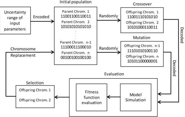
chromosome. The schematic diagram of flow and process of the SGA used is shown

a population of chromosomes. This was one of Talbi’s (2009) recommended

strategies for population initialisation. A pair of randomly selected chromosomes was subjected to the crossover process in order to produce a pair of offspring,

where each offspring was decoded and evaluated based on a fitness function. The offspring with a better fitness value than parent chromosome would replace the

parent chromosome with its own. In a similar manner, the mutation process was

also implemented. This procedure was known as the tournament selection. The

crossover procedure was accomplished by randomly selecting a point in the parent chromosomes and then swapping all the binary digits before the point in a parent

chromosome with the other parent’s chromosome (Reeves, 2003). The mutation process was carried out by randomly selecting binary digit(s) in the offspring’s

chromosome and changing it from 1 to 0 or vice versa. The mutation process was used to help preserve population diversity by preventing a sub-optimal solution at

an early stage of the global search on the input space (Reeves, 2003). The number

of crossovers and mutations was based on the size of population. A complete cycle of the processes resulted in a new generation of population. Multiple generations

would be needed to search for an optimised solution. GA was coded and modified to handle eight input parameters and was also coupled with Richards’ equation.

The code was improved to allow screening of various mutation numbers. Another improvement was the inclusion of termination criteria. The termination of the

simulation was based on pre-set percentage reduction of average fitness function (FF) value stated by Reeves (2003), and also based on pre-set number of times a

percentage reduction value less than the pre-set FF value occcured. The code was improved to include multiple time datasets where the solution (i.e., chromosome) was based upon a sum of FF value of the dataset at various times.

Figure 1: Flow and process schematic of simple genetic algorithm (SGA).

The FF’s objective was to minimise the error between the experimental data

and the simulated results. In this study, the FF used was absolute residual errors as shown below (Zheng and Bennett, 2002):

(8)

where cal_k is the simulated data at cell k ; and obs_k is the analytical solution at cell k.

BA Method

BA was used to imitate the echo location behavior of bats to search for globally-optimum set of input parameters. According to Yang (2010b), BA has three

distinctive features which improved its efficiency. They were frequency tuning,

automatic zooming, and parameter controlling. A population of bats was used to search for the optimum condition, and each bat has its position (x_bat_i) and velocity (v_i ). The success of BA in finding the optimum condition was analogous to a bat finding, locating and reaching a prey or its roosting crevice. The echolocation behaviour begins by the bat emitting a sound pulse that varies in its frequency (f_i ). The loudness of the sound (A_i) reduces as it reaches its target, but the sound pulse rate (r_i ) increases.

The frequency and wavelength combine to provide a constant sound speed in

the air, and thus, if one increased, the other would have to decrease. Yang (2010b)

prefers the parameterization of sound frequency and requires the specification of

minimum (f_min ) and maximum (f_max ) limits of frequency as shown shown below:

f_i = f_min + (f_min - f_max) Rand (9)

where subscript i refers to an individual bat; and Rand is the random number from

the Sobol’ sequence, which has a value between 0 and 1.

The generated frequency would be used to produce a bat’s new velocity (Eq. (10)). It would then update the bat’s existing position to generate a new position (Eq. (11)):

v_it+1 _{= v}

it + (x_batit - x _ batbest ) fi (10)

x_ bat_it+1 _{= x _ bat}

it +vit+1 (11)

where superscript t and t+1 refer to the old (or previous) and new iterations, respectively; x_bat_best is the existing globally best bat position; x_bat_it _{is the}

selected bat position; v_it _{is the existing bat velocity; v}

it+1 is the updated bat velocity after considering the distance between the existing bat and globally best bat

position; and x_bat_it+1 _{is the updated or newly generated bat position that is to be}

Eq. (9) is part of Step 3, refer to Figure 2. Eqs. (10) and (11) are parts of Step 4. In Step 5, the random walk equation provided by Yang (2014) was modified to

the following form: x_ bat_it+1 _{= x _ bat}

best (1 + multiplier) Rdn_num (12)

where multiplier is a fraction value that less than 1; and Rdn_num is a random

number between -1 and 1. Eq. (12) would be executed, only if, a random number that is generated by Sobol’ sequence is greater than sound pulse rate (r_it+1 _{) emitted} by bat as shown below:

(13)

where rio is the initial pulse rate for a bat; γbat is a pulse rate enhancement factor

between 0 and 1; and r_it+1 _{is an updated sound pulse rate for a bat. Eq. (13) indicates}

that the sound pulse rate increases with subsequent updates. Thus, it implies that the likelihood of executing Eq. (12) would be reduced with an increasing number

of updates.

Step 7 would be executed only if: (1) the individual bat fitness value resulting from evaluating either Eqs. (11) or (12), was less than its existing individual bat fitness value; and (2) a generated random number (Sobol’ sequence) was lesser than the loudness value. The loudness value decreases with subsequent updates according to the Eq. (14) shown below:

Ait+1 =αbat Ait (14)

Figure 2: Flow and process schematic of bat algorithm (BA).

where α_bat is a loudness cooling factor between 0 and 1; A_it _{is the initial loudness}

of a bat; and A_it+1 _{is an updated loudness for a bat. The second criterion in}

Step 7 denotes that the probability of replacing an existing individual bat with an improved bat position (with better fitness value) would be reduced with an

increasing number of updates.

Lastly, in Step 8, the globally-optimum position of the bat in each iteration would be stored and compared with other bats’ fitness values. Steps 4 to 8 were repeated until termination criteria were fulfilled. The termination of simulation

was based on a pre-set percentage reduction of average FF value, which was similar to the SGA, and also based on a pre-set number of times a percentage reduction value less than the pre-set FF value was achieved. It was also coded to be able to handle the value of dataset at various times.

RESULTS AND DISCUSSION

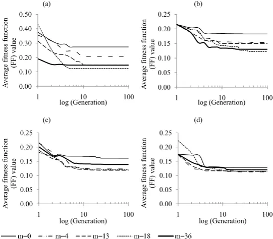
Population size, mutation rate and generation were among the important factors of

SGA (Reeves, 2003). The simulation results were studied for various population

sizes (i.e., 20, 50, 100, 200 and 300) and different mutation rates were applied (i.e., 0, 4, 9, 13, 15, 18, 27, 36, 54, 72 and 90). SGA was set to continue for 100 generations. These mutation rates were applied to each population size. The

fitness value was found to decrease at early generations before reaching a plateau

as the generations continued to increase as shown in Figure 3(a). Decrease in

the fitness value indicated that the simulation results closely matched Philip’s semi-analytical solution from Haverkamp et al., (1977). This trend was observed for different population sizes and also for various mutation rates, as shown in

Figures 3(b)-(d). It thus indicated that a sufficient allocation of generations was required to achieve the desired results. However, allowing the SGA process to continue after the plateauing of the fitness value only wastes computational time. Hence, the SGA code was improved to include termination criteria as suggested by Reeves (2003).

Additionally, a greater population size was found to result in a low fitness value. For instance, a population size of 300 produced fitness values between 0.1123 and 0.2231, whereas a population size of 20 produced finess values between 0.1395 and 0.7686. Similarly, the fitness values for population sizes of 50, 100 and 200 were found located between those of 20 and 300. High population size would result in better simulation results, but required excessive computational time

because increases in the size of the population would also increase the number of

simulation execution for each generation. Thus, finding an optimum population

size was important. Goldberg (1985) suggests that there is an optimal population size for a given chromosome length, but Grefenstette (1986) found it unnecessary. Moreover, for each population size, some mutation rates would result in better simulation results (i.e., low fitness value) as shown in Figures 3(a) to (d). For

example, a mutation rate of 18 resulted in the lowest fitness value of 0.1395 and

0.1239 for population sizes of 20 and 50, respectively. Although previously it was

the mutation rates required to obtain the lowest fitness value were simultaneously

reduced from 18 for a population size of 100 to 4 for a population size of 300.

Similarly, for a population size of 200, the required a mutation rate was only 9. From the observations, it was evident that the fitness value would continue

to decrease with increasing population size. Finding an optimum population size

would require graphical examination of simulation results. A high population size, 300 for instance, provided a slightly better fit on the upper plain of water infiltration front, whilst a low population size, such as 20, improved the lower

plain prediction as shown in Figure 4(a). The simulation results in Figure 4(a) also suggested that there were insufficient data to reproduce the level of upper

and lower plains. Using additional data at the upper and lower plains, a population

size of 50 was found to provide a reasonable prediction and had a fitness value of

0.0122 as shown in Figure 4(b). The SGA unexpectedly failed for a population size of 20, suggesting that the population size used was inadequate.

The SGA method was subjected to additional performance tests that subjected each input parameter to random percentage changes. The evaluation was necessary to prove that the SGA method was able to withstand a variety of

input parameter conditions. The exact percentage variations used are shown in Figure 5(a), whilst Figure 5(b) shows reasonably good prediction results for a

Figure 3: Average fitness function (FF) value for population sizes: (a) 20; (b) 50; (c) 100; and (d) 300. For each population size, different mutation rates (m) were applied as

stated in the legend.

Note: inverse modeling was investigated by varying each input parameter by +20%

from the base value in Table 1. Simulation time was 105_s.

15

(a) (b)

(a) (b)

(c) (d)

(b) (d)

Figure 3: Average fitness function (FF) value for population sizes: (a) 20; (b) 50; (c) 100; and (d) 300. For each population size, different mutation rates (m) were applied as stated in the legend. Note: inverse modeling was investigated by varying each input parameter by +20%

from the base value in Table 1. Simulation time was 105_s. 0.00 0.10 0.20 0.30 0.40 0.50

1 10 100

Ave ra ge fitness f unc tion (F F) va lue log (Generation) 0.00 0.05 0.10 0.15 0.20 0.25

1 10 100

Ave ra ge fitness f unc tion (F F) va lue log (Generation) 0.00 0.05 0.10 0.15 0.20 0.25

1 10 100

Ave ra ge fitness f unc tion (F F) va lue log (Generation) 0.00 0.05 0.10 0.15 0.20 0.25

1 10 100

Ave ra ge fitness f unc tion (F F) va lue log (Generation)

Malaysian Journal of Soil Science Vol. 19, 2015 26

population size of 50 and a mutation rate of 18. Its fitness value was found to

be 0.0978. Thus, it indicated that the SGA method was able to handle random percentage changes in the input parameters.

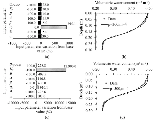
Furthermore, the reliability of the SGA method was evaluated with two

extreme performance tests. The first extreme test reduced all input parameter

values by 100% as shown in Figure 6(a). For instance, θ_r was reduced from 0.124

Figure 4: Water infiltration front with: (a) 28 data points inverse model by different population sizes, i.e., 20, 50 and 300; and (b) 200 data points inverse model by population sizes of 20 and 50. The 200 data points were simulated from a numerical

model and used in the inverse modeling.

Note: p indicates population size and m indicates mutation rate. Simulation time was 105_s.

Figure 5: (a) Random percentage change of the input parameter from the base value (Table 1). (b) Water infiltration prediction at population size (p) of 50 and mutation

rate (m) of 18.

Note: θ_r is the residual volumetric water content, θ_s is the saturated volumetric

water content, K_s is the saturated hydraulic conductivity, θ_{L (initial)} is the initial value of volumetric water content, and α, β, A and B are the fitting coefficients (Eqs. (3) and (4)).

Simulation time was 105_s.

(a) (b)

Figure 5: (a) Random percentage change of the input parameter from the base value (Table 1).

(b) Water infiltration prediction at population size (p) of 50 and mutation rate (m) of 18. Note:

r

 is the residual volumetric water content,s is the saturated volumetric water content, K is s

the saturated hydraulic conductivity, _{L initial } is the initial value of volumetric water content, and

, , A and B are the fitting coefficients (Eqs. (3) and (4)). Simulation time was 105_s. 0.00

0.05 0.10 0.15 0.20 0.25 0.30

0.20 0.30 0.40 0.50

D

ept

h (m

)

Volumetric water content (m3_m-3₎

Data p=50,m=18

-40 -20 0 20 40

Input parameter variation from base value (%)

Input

pa

ra

m

et

er

θL(initial)

Ks

B

A β θs

θr

to zero where this value was used as a low limit (a_i ) in Eqs. (5) to (7). The extreme test would require a population size of 300, as shown in Figure 6(b), to provide

reasonable prediction results at a fitness value of 0.1250. Whilst maintaining the use of the low limit of the first extreme test, the second extreme test increased

the high limit (b_i ), as shown in Figure 6(c), of Eqs. (5) to (7). The extreme test would require at least a population size of 500, which was barely sufficient to provide a reasonable prediction with a fitness value of 0.1763, as shown by Figure 6(d). Hence, a wide range of uncertainty in input parameter value would require

a greater population size (i.e., more than 500) to maintain reasonable prediction results.

In BA, there were a few extra important factors to consider. Apart from the population size and the generations, as in SGA, in BA there were: (1) maximum limits of frequency, f_max , after setting f_min to zero, refer Eq. (9); (2) multiplier, in

Figure 6: (a) Extreme percentage reduction of the input parameter from the base value (Table 1). (b) Water infiltration prediction based on input range of graph (a) at population size (p) of 300 and mutation rate (m) of 4. (c) Extreme percentage reduction

and increase of input parameter from base value (Table 1). (d) Water infiltration prediction based on input range of graph (c) at population size (p) of 500 and mutation

rate (m) of 4.

Note: θ_r is the residual volumetric water content, θ_s is the saturated volumetric water content, K_s is the saturated hydraulic conductivity, θ_{L (initial)} is the initial value of volumetric water content, and α, β, A and B are the fitting coefficients (Eqs. (3) and (4)).

Simulation time was 105_s.

Fitting Constitutive Functions to the Soil Water Flow

2

(a) (b)

(c) (d)

Figure 6: (a) Extreme percentage reduction of the input parameter from the base value (Table

1). (b) Water infiltration prediction based on input range of graph (a) at population size (p) of

300 and mutation rate (m) of 4. (c) Extreme percentage reduction and increase of input

parameter from base value (Table 1). (d) Water infiltration prediction based on input range of

graph (c) at population size (p) of 500 and mutation rate (m) of 4. Note: r is the residual

volumetric water content,s is the saturated volumetric water content, K is the saturated s

hydraulic conductivity, L initial  is the initial value of volumetric water content, and , , A

and B are the fitting coefficients (Eqs. (3) and (4)). Simulation time was 105_s.

0.00 0.05 0.10 0.15 0.20 0.25 0.30

0.20 0.30 0.40 0.50

D

ept

h (m

)

Volumetric water content (m3_m-3₎

Data p=300,m=4 0.00 0.05 0.10 0.15 0.20 0.25 0.30

0.20 0.30 0.40 0.50

D

ept

h (m

)

Volumetric water content (m3_m-3₎

Data p=500,m=4 -100.0 -100.00.0 -100.0 -100.0-100.0 -100.0-100.0 30.05.0 910.1 5.0 35.0 40.0 30.0 22.0

-1000 -500 0 500 1000

Input parameter variation from base value (%) Input pa ra m et er -100.0 -100.00.0 -100.0-100.0 -100.0 -100.0 -100.0 103.0222.6 910.1 400.0 140.8408.5 12,900.0 278.8

-10000 -5000 0 5000 10000 15000

Eq. (12); (3) pulse rate enhancement factor, γ_bat , in Eq. (13); (4) initial pulse

rate, r_io _{, in Eq. (13); (5) loudness cooling factor, α}

bat , in Eq. (14); and (6) initial

loudness, A_it _{, in Eq. (14). In this study’s SGA, there was only mutation rate apart}

from population size and generations. By following a similar procedure to SGA,

those six parameters of BA were calibrated to search for the best FF value. The first stage of calibration was done by repeatedly deviating one parameter at a

time from the default values (Table 2), whilst maintaining all other parameters

unchanged. This was carried out individually on all those six parameters. The

best parameter values (i.e., each parameter with the best FF value) were selected

TABLE 1

The base values of input parameters from Haverkamp et al. (1977) for Yolo light clay.

TABLE 2

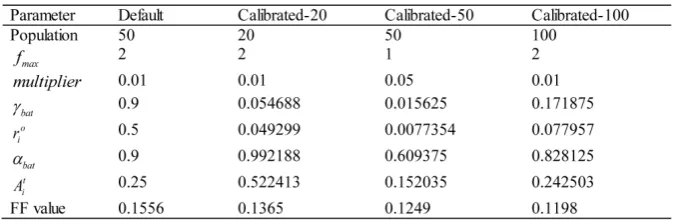
The base (or default) value of input parameters for Bat Algorithm (BA). Parameter values for population 20, 50 and 100 were calibrated.

Goh, E.G. and K. Noborio

12

TABLE 1

The base values of input parameters from Haverkamp et al. (1977) for Yolo light clay.

Parameter Base value

 739

r

 0.124 m3 _m-3

s

 0.495 m3 _m-3

 4

A 124.6

B 1.77

s

K 1.23x10-7 _{m s}-1

 

L initial

 0.2376 m3 _m-3

Notes: ris the residual volumetric water content, sis the saturated volumetric water content, Ksis the saturated hydraulic conductivity, L initial_{ }is the initial value of volumetric water content, and ,

, A and B are the fitting coefficients (Eqs. (3) and (4)). The upper boundary was set to saturated volumetric water content, i.e.,0.495 m3 _m-3_{, and lower boundary was set permeable inflow and outflow}

of water. The data used by Haverkampet al., (1977)fitted to Eq. (3) were obtained from Philip (1969)

and data for Eq. (4) were from Philip (1957).

Notes: θ_r is the residual volumetric water content, θ_s is the saturated volumetric water content, Ks is the saturated hydraulic conductivity, θL (initial)is the initial value of volumetric water content, and α, β, A and B and are the fitting coefficients (Eqs. (3) and

(4)). The upper boundary was set to saturated volumetric water content, i.e.,0.495 m3 _m-3_, and lower boundary was set permeable inflow and outflow of water. The data used by Haverkamp et al., (1977) fitted to Eq. (3) were obtained from Philip (1969) and data for

and used. The process was then performed for other individual parameters. This process was repeated two times. In the second stage of calibration, the fmax and multiplier parameters were fixed for convenience. The remaining four parameters were randomly sorted through using the Sobol’ sequence to account for every possible quad combination. Goh and Noborio (2014) illustrated the spatial coverage of the Sobol’ sequence in two dimensions for two parameters.

In the first stage of calibration, the default condition was found to generate an FF value of 0.1556, and when those six parameters were varied individually

(or individually-calibrated), the lowest FF value of 0.1276 was found and it was

significantly lower (or improved) than that of the default condition. Another

round of searching was carried out using the individually-calibrated values, and it was found to cause deterioration (or increase) in the FF value to 0.1499. The parameter values were not provided in the table. The combined individually-calibrated parameters were unable to generate a good FF value indicating that there were some degrees of interaction between the parameters that could be

exhibiting either antagonistic or synergistic behaviours. This problem was solved

in the second stage of calibration by simultaneously varying four input parameters (i.e., pulse rate enhancement factor, initial pulse rate, loudness cooling factor and the initial loudness). An improved FF value of 0.1365 was found even for a population size of 20 (refer Table 2 for calibration-20), and 0.1249 and 0.1198 at

calibration-50 and calibration-100, respectively. Compared to SGA’s FF values,

which included 200 data points as showed in Figure 4(b), BA’s FF value of 0.1365 was found to outperform SGA’s FF value of 0.4906, for a population size of 20. However, for a population of 50, SGA outperformed BA with respective FF values

of 0.0122 and 0.1249.

For SGA, a calibrated mutation rate was found after eleven trial-and-error

iterations, whilst for BA, the best quad combination was found at the 84th_{, 54}th _and 42nd _{iterations for population sizes of 20, 50 and 100, respectively. Additionally,} if SGA and BA were compared for a population size of 20 without considering the total number of trial-and-error iterations needed to obtain the calibrated

parameter values, corresponding total model executions of 1,040 and 540 were needed, whilst for a population size of 50, model executions needed were 3,400 and 1,650. At this point, BA appears to be more cost efficient than SGA. However, if the total count number of trial-and-error iterations (i.e., the search for

optimising parameter values) were included, the SGA would require only 11,440 model executions, whilst BA would require 45,360 for a population size of 20. Similarly, for a population size of 50, SGA and BA required 37,400 and 89,100 model executions, respectively.

CONCLUSION

The SGA was found to be an effective method to predict a globally-optimum set of input parameter values where the simulation results were found to match

the existing data points closely. A large number of generations were unnecessary as in most cases minimum fitness value was reached in the early generations

(i.e., between 5 and 40). The SGA was solved with termination criteria. Large population size resulted in a low fitness value, thus, suggested better simulation results. SGA required expensive computational time and, therefore, finding

optimum population size was a better approach. In this study, a population size

of 50 was sufficient to provide reasonable simulation results, except when there was an extremely uncertain range of input parameter values where it required an excessive increase in the population size. Additionally, it was found for each

population size, a particular mutation rate applied in order to obtain the lowest

fitness value. Although this value varied for each population size, it was observed

to decrease as the population size increased. Whilst SGA was able to reproduce

sound simulation results, data points at saturation and residual levels were equally important as those of the water infiltration front. It was necessary to perform a

meaningful search of globally-optimum set of input parameter values. Moreover, SGA was found to perform reasonably well under constant increments (+20%) and

random percentage changes in input parameter values. Under extreme cases, as mentioned previously, SGA continued to perform reasonably well at the expense

of higher population sizes and greater computational time. An educated guess to narrow the range limit of input uncertainty would result in better simulation

results, smaller population size and ultimately, require less computational time.

Comparing the SGA to the BA, the latter appeared to perform well at a low population size (i.e., 20) whilst the former was found better at a population size of 50. SGA was the better choice after considering the number of model

executions needed for model calibration, a reasonably small population size without sacrificing FF value, and the number of input parameters that must be

calibrated in order to search for a small FF value. ACKNOWLEDGEMENTS

The authors would like to acknowledge the financial support from Meiji University, Japan and the Ministry of Higher Education, Malaysia and Universiti Malaysia Terengganu. Expressions of sincere thanks also goes to the anonymous reviewers

for their comments on this manuscript.

REFERENCES

Baluja, S. 1994. Population-Based Incremental Learning. A Method for Integrating Genetic Search Based Function Optimization and Competitive Learning. Report

No.CMU-CS-94-163Pittsburgh, PA: Carnegie-Mellon University.

Cedeno, W., and V. Vemuri. 1992. Dynamic multi-modal function optimization using genetic algorithms. Paper presented at the Proc. of the XVIII Latin-American Informatics Conference, Las Palmas de Gran Canaria, Spain.

Chambers, L.D. 1995. Practical Handbook of Genetic Algorithms: New Frontiers.

New York: CRC Press, Inc.

Glover, F., and G.A. Kochenberger. 2003. Handbook of Metaheuristics. New York:

Springer.

Goh, E.G. and K. Noborio. 2013. Sensitivity analysis on the infiltration of water into

unsaturated soil. Paper presented at the Proceedings of Soil Moisture Workshop 2013, Hiroshima University Tokyo Office in Campus Innovation Center.

Goh, E.G. and K. Noborio. 2014. Sensitivity analysis using Sobol’ variance-based method on the Haverkamp constitutive functions implemented in Richards’ water flow equation. Malaysian Journal of Soil Science 18: 19-33.

Goldberg, D.E. 1985. Optimal Initial Population Size for Binary-Coded Genetic Algorithms. TCGA Report.Tuscaloosa, Alabama: University of Alabama. Grefenstette, J. 1986. Optimization of control parameters for genetic algorithms.

IEEE Trans. Syst. Man Cybern. 16(1): 122-128.

Haverkamp, R., M. Vauclin, J. Touma, P.J. Wierengaand G. Vachaud. 1977. A comparison of numerical simulation models for one-dimensional infiltrational. Soil Sci. Soc. Am. J. 41(2): 285-294.

Holland, J.H. 1975. Adaptation in Natural and Artificial Systems. Ann Arbor, MI: University of Michigan Press.

Ines, A.V.M. and P. Droogers. 2002. Inverse modelling in estimating soil hydraulic functions: a Genetic Algorithm approach. Hydrol. Earth Syst.Sci. 6(1): 49-66. doi: 10.5194/hess-6-49-2002.

Kelleners, T.J., R.W.O. Soppe, J.E. Ayars, J. Šimůnek and T.H. Skaggs. 2005. Inverse analysis of upward water flow in a groundwater table lysimeter. Vadose Zone J. 4(3): 558-572.

Latombe, J.C. 1991. Robot Motion Planning. New York: Kluwer Academic Publishers.

Levin, M. 1992. Locating putative protein signal sequences. In: Practical Handbook of Genetic Algorithms: New Frontiers, ed. L. Chambers, Vol. 2, pp. 425-440. New York: CRC Press.

Philip, J.R. 1969. Theory of infiltration. In: Advances in Hydroscience, ed. C. Ven Te, Vol. 5, pp. 215-296.

Philip, J.R. 1957. The theory of infiltration: 1. The infiltration equation and its solution. Soil Science 83(5): 345-358.

Reeves, C. 2003. Genetic algorithms. In: Handbook of Metaheuristics, ed. F. Glover

and G. A. Kochenberger, pp. 55-82. New York: Springer.

Richards, L.A. 1931. Capillary conduction of liquids through porous mediums. Journal of Applied Physics 1(5): 318-333.

Schneider, S., D. Jacquesand D. Mallants. 2013. Inverse modelling with a genetic

algorithm to derive hydraulic properties of a multi-layered forest soil. Soil Research 51(5): 372-389. doi: http://dx.doi.org/10.1071/SR13144.

Shin, Y., B.P. Mohanty and A.V.M. Ines. 2012. Soil hydraulic properties in

one-dimensional layered soil profile using layer-specific soil moisture assimilation

scheme. Water Resources Research, 48, W06529 .

Sobol’ I.M. 1990. On sensitivity estimates for nonlinear mathematical models. Matematicheskoe Modelirovanie 112–118.

Talbi, E.-G. 2009. Metaheuristics: from Design to Implementation. New Jersey: John Wiley & Sons.

Whitley, D. 1994. A genetic algorithm tutorial. Statistics and Computing 4(2): 65-85. doi: 10.1007/BF00175354.

Yang, X.-S. 2014. Chapter 10 - Bat Algorithms. In: Nature-Inspired Optimization Algorithms, ed. X.-S. Yang, pp. 141-154. Oxford: Elsevier.

Yang, X.-S. 2010a. Engineering Optimization: An Introduction with Metaheuristic Applications. New Jersey: John Wiley & Sons.

Yang, X.-S. 2010b. a new metaheuristic bat-inspired algorithm. In: Nature Inspired Cooperative Strategies for Optimization (NICSO 2010), ed. J.R. González, D.A.

Pelta, C. Cruz, G. Terrazas and N. Krasnogor, Vol. 284, pp. 65-74. Springer:

Berlin Heidelberg.

Zheng, C. and G.D. Bennett. 2002. Applied Contaminant Transport Modeling (2nd ed.). New York: John Wiley & Sons.