doi: 10.11648/j.acis.20130105.13
A Comparative Evolutionary models for solving Sudoku
A. A. Ojugo.
1, D. Oyemade.
1, R. E. Yoro.
2, A. O. Eboka.
3, M. O. Yerokun
3, E. Ugboh
31
Department of Mathematics/Computer Sci, Federal University of Petroleum Resources Effurun, Delta State 2
Department of Computer Science, Delta State Polytechnic Ogwashi-Uku, Delta State, Nigeria 3
Department of Computer Sci. Education, Federal College of Education (Technical), Asaba, Delta State
Email address:
[email protected](A. A. Ojugo), [email protected](A. A. Ojugo), [email protected](D. Oyemade), [email protected](R. E. Yoro), [email protected](A. O. Eboka), [email protected](M. O. Yerokun), [email protected](E. Ugboh)
To cite this article:
A. A. Ojugo., D. Oyemade., R. E. Yoro., A. O. Eboka., M. O. Yerokun, E. Ugboh. A Comparative Evolutionary Models for Solving Sudoku. Automation, Control and Intelligent Systems. Vol. 1, No. 5, 2013, pp. 113-120. doi:10.11648/j.acis.20130105.13
Abstract
:
Evolutionary algorithms have become robust tool in data processing and modeling of dynamic, complex and non-linear processes due to their flexible mathematical structure to yield optimal results even with imprecise, ambiguity and noise at its input. The study investigates evolutionary algorithms for solving Sudoku task. Various hybrids are presented here as veritable algorithm for computing dynamic and discrete states in multipoint search in CSPs optimization with application areas to include image and video analysis, communication and network design/reconstruction, control, OS resource allocation and scheduling, multiprocessor load balancing, parallel processing, medicine, finance, security and military, fault diagnosis/recovery, cloud and clustering computing to mention a few. Solution space representation and fitness functions (as common to all algorithms) were discussed. For support and confidence model adopted ϖ1=0.2 and ϖ2=0.8 respectively yields better convergence rates – as other suggested value combinations led to either a slower or non-convergence. CGA found an optimal solution in 32 seconds after 188 iterations in 25runs; while GSAGA found its optimal solution in 18seconds after 402 iterations with a fitness progression achieved in 25runs and consequently, GASA found an optimal solution 2.112seconds after 391 iterations with fitness progression after 25runs respectively.Keywords:
Swarms, Agents, Elitist, Evolutionary Algorithms, Constraints, Fitness Function1. Introduction
Soft Computing (SC) aims to harness the potentials of other disciplines via Artificial Intelligence. Thus, create a synergy dedicated to solve problems by exploiting numeric data and human knowledge simultaneously as mathematical models and symbolic reasoning, yielding a technique that is tolerant to imprecision, uncertainty, partial truth and noise in its data via optimization. Often termed evolutionary programming, SC performs quantitative data processing to ensure qualitative knowledge statements and experience using components such as genetic algorithm (GA), particle swarm optimization (PSO), artificial neural network (ANN) etc to mention a few (Abarghouei, Ghanizadeh and Shamsuddin, 2009).
SC has proven efficient in complex optimization. Ojugo (2012) notes 3-feats in their attempt to explore dynamic processes: (a) Continuous adaptation, (b) Flexibility and (c) Robustness. All evolutionary algorithms are derived from
translating into mathematical models, principles of biological processing in the fastest time to yield implicit and predictive evolution of a model that stems from experience in its ability to recognize data feats and behaviours. And in turn, yield an optimal fitness of high quality and void of overfitting that will constantly affect any solution’s quality (Coello, Pulido and Lechuga, 2002).
1.1. Sudoku Overview
Sudoku is a classical CSP task with variables whose permutation yields a unique solution to satisfy constraints. It is a logic-based combinatorial puzzle of 81-cells in 9X9 grid, each cell contains an integer 1 to 9, and further split into nine 3X3 sub-grids with these constraints in mind:
a.Each row and column of cell is only allowed to contain integers one through nine exactly once
b.Each 3X3 sub-grid is also allowed to contain
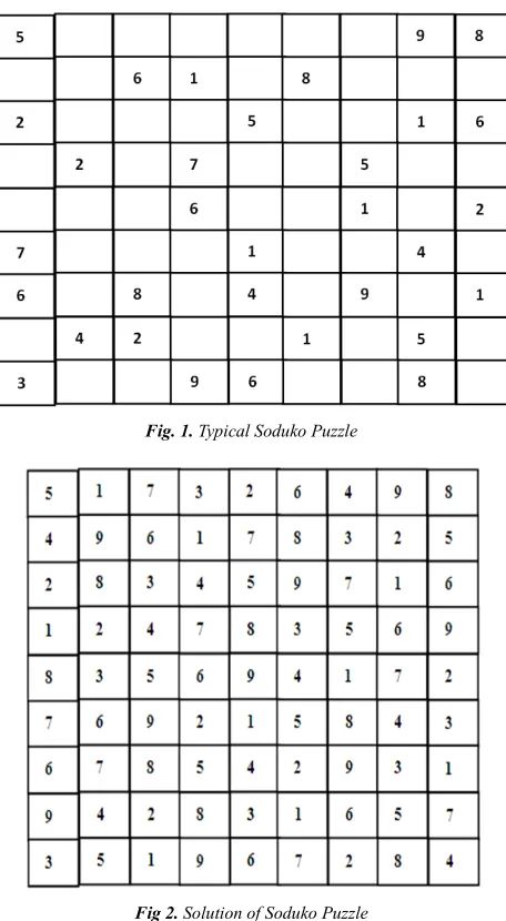
A number of cells are predefined by the puzzle setter, so that each puzzle has a unique solution. Fig. 1 is a typical puzzle, whosesolution is fig 2. Various algorithms have been used to solve Soduko (Santos-Garcia and Palomino, 2007; History of Sudoku, 2013). Some are easily solved via simple logic by mimicking how humans will solve it. Harder puzzles are solved via backtracking algorithms, whose demerit is that its efficiency depends on number of guesses required to solve puzzle (Mantere and Koljonen, 2007). Harder puzzles require longer time to solve, and its solution is via optimization.
Fig. 1. Typical Soduko Puzzle
Fig 2. Solution of Soduko Puzzle
Studies exist that have employed stochastic optimization techniques. A major motivation of this study is that difficult puzzles can be solved efficiently as simple puzzles – due to the fact that the solution space is searched stochastically until a suitable solution is found. Thus, puzzle does not have to be logically solvable or easy for a solution to be reached efficiently (Lewis, 2007; Moraglio and Togelius, 2007). Stochastic methods can be used to find global optima for multipoint dependent tasks for which many local optima
exists that requires systemic search, enabling a space (continuous or encoded discrete) whose solution via hill-climbing method often gets stuck at local minima, a function of their speed in time of finding the solution (global optima). Due to the nature of constraints in Soduko, it is likely to find a solution that satisfies some constraints (solution found is, local optima) but not all of them. Its stochastic nature allows solution space to be searched still (though local optimum is found) until global optima is found (Mantere and Koljonen, 2007).
This study explores the implementation of various stochastic evolutionary optimization methods. Each is implemented and tested on the puzzle in figure 1.
1.2. Solution Space Representation
Fig. 1 consists of 49-empty cells, corresponding to its solution space. Perez and Marwala (2011) notes this solution space can be represented as:
a. First method treats each one of 49 empty cells as separate variable, particle or agent so that each particle or agent requires its own swarm or population. Thus, the solution space consists of 49 separate population groups. The problem with this approach is that each agent can only be operated upon separately, which prevents the possibility of interaction between these individuals or particles. Thus, it is more computationally challenging and demanding.
b. Second, we treat as combination – 49 integers ranging between 1 and 9 (corresponding to the empty cells in fig. 1). As one individual or particle – so that the solution space instead of consisting of 49-different solution groups as in the first case, has only one population with each particle or individual having 49-dimensions or genes. This approach allows for greater interaction amongst the particles or individuals – since algorithm operations are carried out between all possible solutions. This approach is less more computationally demanding. c. Third, represent an individual as a puzzle with all its
cells filled while ensuring that one of the constraints mentioned above is always met. Thus, in initializing a population state, it is ensured that each 3X3 sub-grid in each of the puzzles contains the numbers 1-9 exactly once. Also, any operation carried out on an individual must ensure that this constraint is not violated. This, is less demanding (when compared to the first method) as individual is still represented as a complete puzzle (as opposed to one cell).
1.3. Fitness Function
implement such must ensure that all constraints are met. Its demerit is non-repetition of same integer in same row, column or grid constraints is not guaranteed. A row with nine entries of 5 equals 45 – causing the algorithm to converge to local minimum and not meet all the constraints. Thus, different method is needed (Poli et al, 2006b). The fitness function implemented here involves determining whether an integer is repeated or not present in row, column or sub-grid. A fitness value is assigned to a possible solution, based on number of repeated or non-present integers. The more the repeated or non-present integers there are in a solution’s rows and columns, the higher the fitness value assigned to that solution; while if third approach to solution space representation is considered, then only repetitions in rows and columns are considered; While if second approach is used, then repetitions in the sub-grid contributes to fitness value (Poli et al, 2006b).
1.4. Statement of Problem
Some evolutionary models use backtracking to offer systemic search (in discrete/continuous) spaces via hill-climbing method that often get them stuck at local minima (due to their speed). Thus, hybrids are designed to cub such defects.
1.5. Objective of Study
The study explores Soduko solved via optimization to find a solution space using the third approach in this study to avoid clumsy result presentation via: (a) Cultural Genetic Algorithm (CGA), (b) Genetic Algorithm Gravitational Search Algorithm, and (c) Genetic Algorithm Simulated Annealing respectively.
1.6. Significance of study
Application of this study will yield computational intelligence – veritable tool for dynamic multipoint search in CSPs, applied in areas such as image and video analysis, communication, control, antenna designs, VLSI, data route and compression, simulation, network design and reconstruction, multiprocessor load balancing, OS task scheduling and resource allocation, parallel processing, power generation, medical and pharmaceutical, finance and economics, security and military, engine design and automation, system fault diagnosis and recovery, forecasting and predictions, cloud and clustering computing etc.
1.7. Limitations of Study
Hybrid, though difficult to implement – are used to provide a means for better selection of search space, encoded via structured learning (to address the general problem of determining existing statistical dependencies amongst data variables) and yield better generation with crossover, mutation and temperature schedules etc.
2. Cultural Genetic Algorithm (CGA)
CGA is an evolutionary technique with individuals influenced both genetically and culturally (Reynolds, 1994), whose background is built on genetic algorithm (GA) as thus:
2.1. Genetic Algorithm
GA is a population optimization inspired by Darwinian evolution and genetics (survival of fittest and natural selection). It consists of a population (set of numeric data) chosen for natural selection that consists of potential solutions to a specific task with each potential solutions referred to as an individual (combination of genes). An optimal combination of genes can lie dormant in the population (from a combination of individuals). An individual with a genetic combination close to the optimal is described as being fit (Hassan and Crosswley, 2004).
A new pool is created by mating two individuals from the current pool. The fitness function is then applied to determine how close an individual is to the optimal solution. The selection function ensures that the genetic data from the fittest individuals is passed down to the next generation or pool – so that a fitter pool emerges. Eventually, the new population (as newer pools are created) will converge on the optimal solution or gets close to it as possible. GA operations are carried out in four steps namely:
a. Initialize – encodes chromosomes into a format suitable for natural selection and many encoding modalities exists (each with its own merits and demerits). An individual in population can be represented in binary (which requires more bits to do so). But, if decimal is used – it allows greater diversity in chromosome representation and greater variance of subsequent generations (Perez and Marwala, 2011). An issue with binary encoding is that populations are not naturally represented in binary due to length as it is computationally more expensive (Ojugo, Eboka, Okonta, Yoro and Aghware, 2012).
Another allows individual to be encoded as floating point numbers or its combination and is far more efficient than binary encoding. Values encoded are similar with character and commands to represent
an individual. Encoding scheme encodes data – so
that each solution set consist candidates encoded as fixed length vector in one or more pools of different types. The fitness function sees a solution set from various candidates evaluated, to determine its goodness of fit. If a solution is reached, function is
good; else, is bad and not selected for crossover.
If A then B,
Support = |A and B| / N Confidence = |A and B| / |A|
Fitness = w1 * support + w2 * confidence
b. Selection – First, a fitness function is used to determine how close an individual is to an optimal solution. After which, individuals are selected for mating. Two selection methods are: (a) Roulette method first sums the fitness of all individuals. Then, selects random number between 0 and the summed result. The fitness’s are summed again until the random number is reached or just exceeded, from which last individual to be summed is selected, and (b) tournament selects a random number of the individuals in pool and the fittest individual is selected. The larger the number of individuals selected, the better the chances of selecting a fittest individual. It continues until one is chosen, from last two or three solutions remaining, to become selected parents to create the new offspring. Selection ensures that the fittest individuals are selected and more likely chosen for mating but also allows for less fit individuals from the pool and the fittest to be selected. A selection function which only mates the fittest is termed elitist and often leads to the algorithm converging at a local optima. Here, the tournament algorithm is adopted (it is easier and more efficient to code) as it works on parallel architectures, allowing selection pressure to be easily adjusted (Ojugo et al, 2012) as thus:
Algorithm: Tournament Selection {} 1. Input: Population of chromosome
2. Output: Selected Chromosome for crossover 3. Randomly select 3-chromosomes from pool 4. Pick best 2-solution based on fitness value 5. Return the selected two solution
6. Apply Crossover | Select best solution as parent c. Crossover – involves the reproductive process in
which two individuals exchange their genetic materials to yield a new, fitter individual while ensuring that genes of fit individuals are mixed in an attempt to create a fitter new generation. There are various types of crossover depending on encoding type, two of which are stated as: (a) simple crossover on binary encoded pool, involves choosing multi- or particular-point and all genes are from one parent, and (b) arithmetic crossover in which the new pool is created by adding percentages of one individual to another (Kilic and Kaya, 2001; Ojugo et al, 2012).
d. Mutation – A child’s chromosome, gene sequence is
slightly altered by either (changing its genes or its sequence) – to ensure the pool converge to a global minimum (instead of local optimum). Algorithm stops once an optima is found. Though computationally expensive, GA can also stop when
a number of new pools are created or once no better solution is found. A gene may or may not change depending on mutation rate. Mutation improves diversity needed in reproduction (Ojugo et al, 2012).
Algorithm for Mutation 1. Input: A chromosome rule
2. Output: Mutated solution, a fns of mutation rate 3. Set mutation threshold (between 0 and 1) 4. For each network attribute in chromosome 5. Generate a random number between 0 and 1 6. If random number > mutation threshold then 7. Generate Random value for N-Queen 8. Set solution attribute value with 9. Generated attribute value 10. End if
11. End For Each
2.2. Cultural GA (CGA)
Cultural GA is one of the many variants of GA with a belief space categorized as: (a) Normative (where there is a particular range of values to which an individual is bound), (b) Domain (data about the domain of the task is available), (c) Temporal (data about events in the space is available) and (d) Spatial (topographical data of space is available).
In addition to a belief space, an influence function is needed for CGA (Reynolds, 1994) to form interface between the pool and belief space, to help alter individuals in the pool to conform to its belief space. CGA is chosen, as the model must yield individuals that cannot violate its belief space and reduces number of possible individuals GA needs to generate until an optimum is found. Thus, it is best for Sudoku than other variants (Mantere and Koljonen, 2007). Two CGA methods used in Sudoku:
selected for reproduction via tournament, to determine which individuals will mate.
In reproduction, both crossover (simple single point) and mutation is carried out – in which a number between 1 and 49 is randomly generated from a Gaussian distribution, corresponding to the point of crossover. All genes before this point come from one parent; while the other parent contributes the rest. A new individual, whose genetic makeup is a combination of both parents is thus, reproduced. The new individual also undergoes mutation from which three random genes are selected for mutation and are allocated new random values that still conforms to the belief space. The new individuals replace ones in the pool, with low fitness values (creating a new pool). This continues until an individual with a fitness value of zero (0) is found – to imply that the solution to the puzzle has been reached (Cantu-Paz and Goldberg, 2000).
b. Second – uses third solution space (each individual
is a complete puzzle: each 3X3 grid in each puzzle contain numbers 1 to 9 exactly once so that each 3X3 grid is a gene). Pool of 100 such individual randomly initialized and their fitness computed. The best individual and fitness in the pool at each generation is tracked. The fitness function as described above is used where only repetitions in the rows and columns, contributes to an increase in the fitness value. Thus, no repetitions in the grid as this will also help ensure each contains genes that conform to its belief space which are: (1) Normative (each 3X3 grid contains entries 1 and 9), (2) Domain (each 3X3 grid contain integer entries), (3) Spatial (each 3X3 grid must have integers 1 to 9 just once), and (4) temporal (with mutation, it cannot alter fixed cell values).
This process only implements mutation on each individual separately so that in a 3X3 grid (randomly selected), two unfixed cells in grid are
randomly selected and switched. During
reproduction, the mutation is applied on each individual population. Number of mutation applied on an individual depends on how far CGA has progressed (how fit is the fittest individual in the
population). Thus, number of mutations
implemented equals the fitness of the fittest individual divided by 2. If fittest individual equals 31, number of mutation equals 16.
Thus, at initialization – it is ensured that the first three (3) beliefs are met; while mutation ensures the fourth belief is met. In addition is an influence function in which best fitness helps influence how many mutations takes place. Thus, knowledge of solution (how close puzzle is from being solved) has direct impact on how the algorithm is implemented; and thus, the algorithm terminates
when the best individual has a fitness of 0 – to imply that the solution has been found (Reynolds, 1994).
3. GA-Gravitational Search (GAGSA)
GAGSA is a powerful optimization method, which explores GA’s parallel ability to search a space via multiple individual and GSA’s speed and flexibility in finding a better optimal point even when a local minimum is found. Both are essential to find solution, to a Sudoku task (Perez and Marwala, 2011)
3.1. Gravitational Search Algorithm
GSA is based on laws of gravity and motion of isolated masses, with each mass representing a solution space and states that particle attracts each other and gravitational force between them, is directly proportional to their masses product and inversely proportional to their distance. Thus, an agent’s performance depends on its mass (agents with heavier masses attracts those of smaller masses). GSA uses exploration to navigate its space and guarantee the choice of values by these agents are not violated; and uses exploitation to find optima in shortest time – with agents of heavier masses, moving slowly in order to attract those of lesser mass (Ojugo, 2012). Agents are randomly initialized. At time t, a gravitational force of mass j acts on mass i based on Rij Euclidean distance between any two masses as thus:
(1)
G (gravitation constant) decreases in time to control its accuracy with ε is small constant. Total force is:
∑ , ! (2)
rand – randomizes agents’ initial states at intervals [0,1]. The acceleration of agent i, at time t in dimension d is directly proportional to force acting on that agent, and inversely proportional to its mass, given by:
" #
$
(3)
Next agent’s velocity is a function of its current velocity and its current acceleration computed as:
% & 1 % & " (4)
& 1 % & 1 (5)
Vid(t) is agent velocity in dth dimension at time t, and rand is between [0,1]. Masses are calculated via fitness function, as agents of heavier masses keeps attracting those of lesser mass. Masses are updated:
( # ) *+,
) *+, (6)
worst(t) indicates strongest and weakest agent according to fitness. For minimization task via reverse engineering, best(t) and worst(t) are defined as:
-./ min 3!,4..67 8 (7)
9: / max 3!,4..67 8 (8)
At start, agents are located as solution points in the search space such that with each cycle, the positions and velocities of agents are updated via Eq. (4) and (5), and masses M is updated via Eq. (6). The iteration is stopped when an optimal is found. Thus, we seek agents of lower masses (reverse engineering).
3.2. GAGSA as in Sudoku
The initial use of GA will help achieve a low fitness – so that once a better individual is not found by GA after a number of generations, the best individual is chosen for a series of random walks via its structured learning till an optimal solution is found. Factors defined for GAGSA includes (with GA), how many number of runs is there, how is population representation, its size and reproduction function – must be addressed.
As used in Sudoku, a population of 10 puzzles are initialized to represent the third solution scheme of section 1.2 is met with each 3X3 grid containing integer 1 to 9 exactly once. The reproduction function for the GA, only mutation is implemented to randomly select a grid and randomly swap two unfixed cells in the grid. Number of mutations corresponds to best fitness; and, best fitness and individual, is tracked until a fitness of 2 is found (experimentally, it is found that GA found a fitness of 2 very quickly). Perez and Marwala (2011) notes GA found individuals with low energy of 2, which enters a GSA cycle fairly late. Thus, if GA yields an individual with fitness close to optimal – gravitational force and force acting on each particle is computed with Eq. (1) and (2), to accept individuals with masses lower or equal to current (state’s) mass. This runs, until a state with the mass of 0 is reached (solution is found).
4. GA-Simulated Annealing (GASA)
A background of simulated annealing as thus:
4.1. Simulated Annealing
SA as inspired by annealing process used to strengthen glass and crystals – such that a glass is heated until it liquefies and then, allowed to cool slowly so that the molecules settles into lower energy states. Thus, it rather tracks and alters the state of an individual, continuously evaluating its energy using an energy function. Its optimal point is found by running series of Markov chain under different thermodynamic states: neighbouring state is determined by randomly changing an individual’s current
state by implementing the neighbourhood function. If state with lower energy is found, individual moves to it. Else, if neighbourhood state has a higher energy, then the individual will move to that state only, if an acceptance probability condition is met. If not met, the individual remains at the current state (Perez and Marwala, 2011).
The acceptance probability is difference in energies between current and neighbouring states, and temperatures. Temperature is initially set high, so individual is more inclined towards higher energy state – allowing the individual to explore a greater portion of the space and preventing it from being trapped in local optimum. As algorithm progresses – temperature reduces with cooling so that individuals converge towards lowest energy states and thus, an optimum point (Perez and Marwala, 2011). The algorithm is as thus:
Simulated Annealing Algorithm:
1. Initialize an individual state and energy 2. Initialize temperature
3. Loop until temperature is at minimum
4. Loop until maximum number of iterations reached
5. Find neighbourhood state via neighbourhood
function
6. If neighbourhood state has lower energy than
current
7. Then change current state to neighbouring state
8. Else if the acceptance probability is fulfilled
9. Then move to the neighbouring state
10. Else retain the current state
11. Keep track of state with lowest energy
12. End inner loop
13. End outer loop
4.2. Hybrid GA-SA
GASA is a powerful model that combines GA’s parallel search to explore the space via multiple individuals and SA’s flexibility to find a better optimal point, even when a local minimum is found. Both are essential in finding solution to a Sudoku task (Perez and Marwala, 2011).
Initial use of GA helps achieve a low fitness – so that once a better individual is not found after a number of runs, the best individual is chosen for a series of random walks until an optimal solution is found. These factors must be defined for GASA: (a) On GA: number of runs, population representation, size and reproduction function, and (b) On SA (with GA complete), SA is run on the fittest individual until a solution is found and what is the neighbourhood size and function.
single Markov chain is run). The number of mutations will correspond to the best fitness, with the best fitness and individual tracked until a fitness of 2 is found (experimentally, it is found that GA found a fitness of 2 very quickly). Perez and Marwala (2011) notes since GA found individuals with low energy, they enter into the SA cycle fairly late so that no temperature schedule is needed. Instead, a simple moderated Markov chain is used, which accepts the states with energies that are lower or equal to the current state’s energy. This runs until the state with the energy of 0 is reached (solution is found). The SA and GA shares the same fitness function; while SA neighbourhood function is same as mutation function used in GA.
5. Result Discussion
After testing all three (3) models on figure 1 puzzle, the results are presented as follows:
5.1. CGA Result
CGA took 32 seconds to find the solution after 188 iterations or generations (at best). CGA was run 25 times (to eradicate non-biasness) and it was able to find an optimal solution every time – and the time taken varied significantly between 32 seconds and 8 minutes, as CGA convergence time depends on how close the initial population is to the solution and on the random mutation applied to the individuals in the pool and is supported by Perez and Marwala (2011).
5.2. GAGSA Result
GSAGA solves puzzle (at best) 18seconds after 402 iterations with a fitness progression achieved across GSA and GA as well. The GA cycle achieved a fitness of 2 in 90 iterations and GSA implemented a gravitational pull and mass update of 332 iterations before finding a solution. GSAGA was run 25 times and solved the puzzle each time on a range between 12seconds and 11minutes – due to its stochastic nature so that convergence time depends on initialization and gravitational pull cum mass updates.
5.3. GASA Result
GASA solves puzzle at 2.112seconds after 391 iterations with fitness progression across GA and SA. GA achieved a fitness of 2 in 90 iterations and SA used Markov chain of 301 iterations to find a solution. With 25 runs, GASA solved puzzle every time on a range between 4seconds and 3minutes – due to its stochastic nature as convergence time depends on initialization as well as the random swaps and is supported by Perez and Marwala (2011).
6. Conclusion / Recommendation
The Sudoku is solved efficiently via stochastic method: three of which are used in this work. Solution space
representation and fitness functions (as common to all algorithms) were discussed, and support/confidence model adopts ϖ1=0.2 and ϖ2=0.8 to give better convergence. Other values, led to a slower convergence or non-convergence.
References
[1] Abarghouei, A., Ghanizadeh, A and Shamsuddin, S., (2009): Advances in soft computing methods in edge detection, J. Advance Soft Comp. Applications, ISSN: 2074-8523, 1(2).
[2] Cantu-Paz, E and Goldberg, D.E., (2000): Efficient parallel genetic algorithms: theory and practices, Computer methods in applied mechanics and engineering, 186(2-4), pp 221-238.
[3] Coello, C. A., Pulido, G. T and Lechuga, M.S., (2002): Handling multiple objectives with particle swarm optimization, Evo. Comp., Vol. 8, pp 256–279.
[4] Hassan, R and Crosswley, W., (2004): Variable population-based sampling for probabilistic design optimization and with a genetic algorithm, AIAA-2004-0452), 42nd Aerospace Science meeting, Reno, NV.
[5] Hassan, R., Cohanin, B., De Wec and Venter, G., (2006): Comparism of PSO and GA, American Institute of Aeronautic and Astronautics (AIAA-2006), 44th Aerospace Science meeting, Washington–DC.
[6] Heppner, H and Grenander, U (1990): A stochastic non-linear model for coordinated bird flocks, In Krasner, S (Ed.), The ubiquity of chaos, (pp. 233–238). Washington: AAAS.
[7] History of Sudoku, Conceptis Editoria, [online]: www.conceptispuzzle.com/articles/sudoku, last accessed 17-01-2013.
[8] Kilic, A. and Kaya, M.A (2001): A new local search algorithm based on genetic algorithms for the n-queens problem, Proc. Genetic and Evo. Comp. conf. (GECCO-2001), 158 – 161
[9] Lewis, R., (2007): Metaheuristics can solve Sudoku, J. Heuristics Archive, 13(8), pp 387 – 401
[10] Mantere, T and Koljonen, J., (2007): Solving and rating Sudoku puzzles via genetic algorithm, Proc. Congress on Evol. Comp.,1382-1389.
[11] Moraglio, A and Togelius, J., (2007): Geometric particles swarm optimization for Sudoku puzzle, http://julian.togelius.com/Moraglio2007Geomet-ric.pdf, last accessed 16-January-2013.
[12] Ojugo, A., Eboka, A., Yoro, E., Okonta, E and Aghware, F.O., (2012): Genetic algorithm rule-based intrusion detection system, J. Emerging Trends in Comp. Info. Syst., ISSN: 2079-8407, 3(8), pp 1182-1194
[14] Perez, M and Marwala, T., (2011): Stochastic optimization approaches for solving Sudoku, Proc. IEEE Congress on Evo. Comp., pp 256–279, Vancouver: Piscataway.
[15] Poli, R., Wright A., McPhee, N and Langdon, W., (2006b): Emergent behaviour, population based search and low-pass filtering, Proc. on Comp. Intelligence and Evo.Comp., pp395-402, Vancouver: Piscataway
[16] Reynolds, R., (1994): An introduction to cultural algorithms, Proc. of 3rd Annual Conf. on Evo. Programming, River Edge: New Jersey, World Scientific, pp 131-139.