Theoretical Study of the Electrostatic Lens Aberrations of
a Negative Ion Accelerator for a Neutral Beam Injector
Kenji MIYAMOTO and Akiyoshi HATAYAMA
1)Naruto University of Education, 748 Nakashima, Takashima, Naruto-cho, Naruto-shi, Tokushima 772-8502, Japan
1)Faculty of Science and Technology, Keio University, 3-14-1 Hiyoshi, Kohoku-ku, Yokohama 223-8522, Japan
(Received 25 July 2008/Accepted 21 December 2008)
Aberrations due to the electrostatic lenses of a negative ion accelerator for a neutral beam injector and the space charge effect are theoretically investigated. A multi-stage extractor/accelerator is modeled and the aberration coefficients are numerically calculated using the eikonal method, which is conventionally used in electron optics. The aberrations are compared with the radii of a beam core with good beam divergence and a beam halo with poor beam divergence. H−beamlet profile measurements give the 1/eradii of the beam core and beam halo of 5.8 mm (beam divergence angle: 6 mrad) and 11.5 mm (beam divergence angle: 12 mrad), respectively. When the beam divergence angle of the beam core is 5 mrad and the beam energy is 406 keV, the aberrations due to the electrostatic lenses are less than a few millimeters, thus are less than the radii of the beam core and beam halo. The geometrical aberrations due to the space charge effect (negative ion current density: 10 mA/cm2), however, are estimated to be much larger than the radius of the beam halo. Although the aperture
radii of the grids are not taken into account in this estimation, the results indicate that the space charge effect is an important factor in the aberration or beam halo in a negative ion accelerator.
c
2009 The Japan Society of Plasma Science and Nuclear Fusion Research
Keywords: nuclear fusion device, NBI, accelerator, negative ion beam, aberration, electrostatic lens DOI: 10.1585/pfr.4.007
1. Introduction
A negative ion-based neutral beam injection system (N-NBI system) is a promising candidate for plasma heat-ing and current drive of fusion reactors such as the interna-tional thermonuclear experimental reactor (ITER). ITER requires the N-NBI system to provide high power neutral beams with a beam energy of 1 MeV and beam power of 50 MW using three injectors [1–4].
A negative ion source/accelerator that can produce negative ion beams with high current and power is the key component for the N-NBI system. Negative ion beams with a beam energy of 1 MeV, beam current of 40 A, and beam current density of 20 mA/cm2 are required for the
ITER-NBI [1–4]. To suppress the geometrical loss of neg-ative ion beams and heat loads in the beamline, NB duct, and injection port, it is essential to accelerate the negative ion beams with good beam optics.
As for the H− beam optics, Holmes et al. measured the H− ion beamlet produced with a pure volume source, and reported that the profile consists of two Gaussian portions—a beam core with good divergence and a beam halo with poor divergence [5]. H− ion beamlet profiles with these two Gaussian portions were confirmed with the 400 keV negative ion accelerator [6, 7]. In the ITER-NBI, the beamlet is also considered to consist of the beam core
author’s e-mail: [email protected]
(<5 mrad) and beam halo (>15 mrad), and the ITER-NBI is designed on the basis that the power fraction of the beam halo is estimated to be 15% of the total beam power [8].
It is well known that the effects of aberrations degrade the charged particle beam optics. Generating aberrations is inevitable when the charged particle beams are extracted, accelerated, transmitted, and focused with electrostatic and magnetic fields. For charged particle optical instruments in the field of the electron microscopes and focused ion beam systems, aberrations degrade the focused beam spot, limiting the spatial resolution of these instruments. There-fore, in developing of the charged particle optical instru-ments, many authors have studied the aberrations due to the electrostatic lens, magnetic lens, and space charge ef-fect [9–17].
In the ITER-NBI design, there is no specification for an acceptable level of aberration. However, very lit-tle is known about the aberrations in the negative ion source/accelerator for the N-NBI system. In fact, the aber-rations arise from the electrostatic lenses, magnetic lenses produced by the magnetic filter and permanent magnets for electron suppression, the plasma-beam boundary, and the space charge effect. Moreover, the aberrations are con-sidered to be one of the reasons for the beam halo. As described above, although the beam halo was verified ex-perimentally in the H− beamlet profile [5–7], its physical
c
mechanism is not clear.
The main purpose of the present study is to investi-gate the aberrations in the extractor/accelerator theoreti-cally. This paper focuses on aberrations due to the electro-static lenses and the space charge effect. The well-known eikonal method [17–21] is used to calculate these aberra-tions, and the calculated aberrations are discussed quanti-tatively by comparing them with the radii of the beam core and beam halo, as reported in Refs. [6, 7].
This article is constructed as follows: the calculation models for the electrostatic potential, negative ion beam trajectory, and aberration are described in Sec. 2: the cal-culation results are shown and discussed in Sec. 3: and a summary is given in Sec. 4.
2. Calculation Model
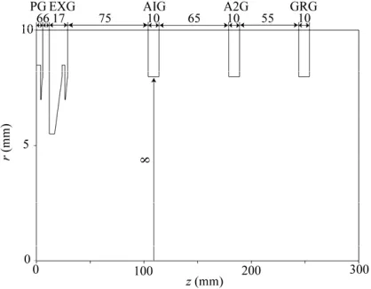
Figure 1 shows a cross-sectional view of the extrac-tor and acceleraextrac-tor for the present model. Figure 1 (a) shows an overall view of the extractor and accelerator and Fig. 1 (b) shows a magnified view of the extractor. The ex-tractor and accelerator are multi-aperture and multi-stage types. Negative ions are extracted and accelerated electro-statically.
The extractor consists of a plasma grid (PG) and an ex-traction grid (EXG), which have the same structure as the extractor of the negative ion source for ITER-NBI. In or-der to extract negative ions with good beam optics, the PG and EXG are shaped to produce convergent electrostatic lenses in the extractor. Permanent magnets are embedded in the EXG to suppress the electrons extracted along with negative ions. These magnets produce the magnetic lens. In the present model, this magnetic lens is not taken into account.
The accelerator consists of a first acceleration grid (A1G), second acceleration grid (A2G), and grounded grid
Fig. 1 Cross-sectional view of the extractor and accelerator in the present model. (a) Overall view of the extractor and accelerator. (b) A magnified view of the extractor.
(GRG). The aperture diameter, gap length, and number of acceleration stages are the same as those of the accelerators for JT-60U N-NBI [22, 23] and the 400 keV negative ion source [24, 25]. The gap length is designed to be progres-sively shorter in the downstream stages to form converging electrostatic lenses at each grid aperture, and thereby sup-press beam divergence due to the space charge effect.
2.1
Calculation of electric field
To calculate the electric field in the extractor and ac-celerator, Laplace’s equation is solved using a finite differ-ence method with successive over-relaxation.
1) The extractor and accelerator are modeled to be rota-tionally symmetric. Ther-axis is taken to be the direction of the beam radius, whereas thez-axis is taken to be the direction of beam acceleration.
2) The mesh sizes are 0.025, 0.05, 0.1, and 0.2 mm. The minimum mesh size of 0.025 mm is approximately the De-bye lengthλDin the extraction region of the negative ion
source. The Debye lengthλDcan be estimated as follows:
at an arc power of 10 kW, the ion saturation current in the extraction region is approximately 200 A/m2[26, 27].
As-suming that the electron temperatureTe is 1 eV, and the
ratio of the electron density to the ion density is 0.9 [28], one obtains
ne=0.9
× 200
1.60×10⁻¹⁹×exp(−0.5)×1.60×10−19×1/1.67×10−27
=1.9×10¹⁷m−3.
Therefore,λDis estimated to be 0.017 mm.
3) The entrance of the PG is set to bez = 0 mm. The position where the negative ion beamlet profiles was mea-sured, as in Refs. [6, 7], corresponds toz=1214 mm in the present model. Modeling to this position incurs high cal-culation costs. Since an electric field generally penetrates into the field-free region by a distance of the diameter of an aperture (at most), the calculation region is modeled up to z=270 mm, i.e., 16 mm downstream from the GRG exit. The regions ofz > 270 mm are assumed to be field-free (E=0).
4) The plasma-ion boundary is equivalent to an object planez=zo. Except for the electrodes, the mesh regions
ofz≤zo−dhare assumed to be the plasma region, and the
electrostatic potential is set to be zero.
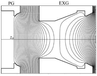
5) The shape of the plasma-beam boundary will result in the aberrations because the plasma-beam boundary has a lens effect [29]. In the present model, the plasma-beam boundary is assumed to be flat. Thus, aberrations caused by the shape of the plasma-beam boundary are not con-sidered. An example of equipotentials in the extractor is shown in Fig. 2.
Fig. 2 Example of equipotentials in the extractor.
Table 1 Voltages of each grid in the extractor and accelerator.
Grid PG EXG A1G A2G GRG
Voltage (kV) 0 6.40 139.73 273.07 406.40
of 406 keV, as shown in Table 1. The electrostatic lenses in the present model are similar to those of the 400 keV negative ion accelerator.
2.2
Calculation of ion beamlet trajectory
The paraxial ray equation of the negative ion beamlet is given by [15]uG+ φ 2φuG+
φ+ρ
4φ uG=0, (1)
where φ is an electrostatic potential, and ρ is the space charge density for the H−ion beamlet. In Eq. (1), primes signify differentiation with respect to z. The paraxial ray equation is solved using the fourth-order Runge-Kutta method.
The two fundamental solutions of Eq. (1) are given as g=g(z) (g-trajectory) andh=h(z) (h-trajectory) with the following initial conditions at the object planez=zo:
g(zo)=1, g(zo)=0, h(zo)=0, h(zo)=1. (2)
The solution of the paraxial ray Eq. (1) is given by uG=A1g(z)+A2h(z), (3)
whereA1andA2are the constants.
In general, the optical properties of the electrostatic lenses can be evaluated from the g-trajectory and h-trajectory (see Fig. 3):
• The position of an image plane z = zi is estimated
fromh(zi)=0.
• MagnificationMis defined byg(zi)=|M|.
• Focal length fiis given by fi=−
1 g(zi).
• The position of a focal planez=zFi is given byzFi =
zi+M fi.
• The position of a principal planez = zhi is given by
zhi=zFi−fi.
Moreover, the aberration due the electrostatic lenses and the space charge effect can be estimated with the two fundamental solutions, as will be shown in the next section.
2.3
Estimation of aberration due to the
elec-trostatic lenses
The aberration of the electrostatic lenses is calculated using the eikonal method, which is conventionally used in electron optics [17–21]. As the high order derivatives such asφ(3)andφ(4)cause inaccuracies in numerical integration,
these high order derivatives are excluded using Seaman’s procedure [30–32].
The space charge effect is not taken into account in the following.
2.3.1 Geometrical aberration
From the eikonal method (see Appendix), the geometrical aberrationu3(zi) referred to the object side is given as
u3(zi)=M
C(o)s uo2u¯o+C (o)
l uou¯ouo+C(o)r uo2u¯o
+C(o)a u2ou¯o+C (o)
f uou¯ouo+C (o) d u
2 ou¯o
, (4) In Eq. (4), the aberration is expressed in terms of the beam trajectory and beam divergence angle at the object plane, i.e.,uG(zo)=uo,uG(zo)=uo. Moreover, ¯uoand ¯uo
are the complex conjugates ofuoanduo, respectively. The
geometrical aberration coefficients ofC(o)s ,C(o)l ,Cr(o),Ca(o),
C(o)f ,Cd(o)are defined as follows: C(o)s : a coefficient of spherical aberration
C(o)l ,Cr(o): a coefficient of coma
C(o)a : a coefficient of stigmatism
C(o)f : a coefficient of field curvature C(o)d : a coefficient of distortion
In terms ofg(z) andh(z), the aberration coefficients of C(o)s ,Cl(o),C(o)r ,C(o)a ,C(o)f ,Cd(o)are given as follows:
C(o)s =
1 32
zi
zo
φ φo
F1h4+F2h3h+F3h2h2
dz
− 1
32
φ
φo E1h4+E2h3h+E3h2h2+E5hh3
zi
zo
,
1 2C
(o) l =C
(o) r =
1 128
zi
zo
φ φo
4F1gh3
+F2h22gh+(gh)+2F3hh(gh)
dz
− 1
128
φ φo
4E1gh3+E2h22gh+(gh)
+2E3hh(gh)+E5h2
2gh+(gh)zi
zo
C(o)a = 1 64 zi zo φ φo
2F1g2h2−F2gg(gh)+2F3ghgh
dz
− I2
128√φo
zi
zo
F4
√φdz− 1 64
φ φo
2E1g2h2
+E2gh(gh)+2E3ghgh+E5gh(gh)
zi
zo
,
C(o)f = 1 64 zi zo φ φo
4F1g2h2+2F2gh(gh)+F3(gh)2
dz
− I2
128√φo
zi
zo
F4
√φdz− 1 64
φ
φo
4E1g2h2
+E2gh(gh)+E3(gh)2+2E5gh(gh)
zi
zo
,
C(o)d = 1 128 zi zo φ φo
4F1g3h+F2g2(2gh+(gh))
+2F3gg(gh)
dz− 1 128
φ φo
4E1g3h+E2g22gh
+(gh)+2E
3gg(gh)+E5g22gh+(gh)
zi
zo
,
(5) where
I= φgh−gh, E1=
1 2
φφ φ2 +φ
(3),
E2=−
4φ φ ,
E3=−
8φ φ , E5=−16,
F1=−
3 4
φ2φ
φ3 +
5 2 φ φ 2 ,
F2=
10φφ φ2 ,
F3=12
φ
φ
2
. (6)
On the other hand, the geometrical aberrationu3(zi)
referred to the image side is given as u3(zi)=C(i)s ui
2
¯
ui+Cl(i)uiu¯iui+Cr(i)ui 2
¯
ui+Ca(i)u2iu¯i
+C(i)f uiu¯iui+C (i) d u
2
i. (7)
In this case, the aberrations are expressed in terms of the beam trajectory and beam divergence angle at the image plane, i.e.,uG(zi)=ui,uG(zi)=ui. Moreover, ¯uiand ¯uiare
the complex conjugates ofuiandui, respectively.
The relation between the aberration coefficients in Eqs. (4) and (7) is given by
C(i)s =M4ξi3C (o) s ,
C(i)l =2M2ξ2i
M fo
Cs(o)+C(o)r
,
C(i)r =M2ξi2
M fo
C(o)s +C(o)r
,
C(i)a =ξi⎧⎪⎪⎨⎪⎪⎩C(o)a +
2MC(o)r
fo
+M2 f2
o
C(o)s ⎫⎪⎪⎬⎪⎪⎭,
Cf(i)=ξi⎧⎪⎪⎨⎪⎪⎩C(o)f +
4MCr(o)
fo +
2M2
f2 o
Cs(o)⎫⎪⎪⎬⎪⎪⎭,
Cd(i)= 1 M2C
(o) d +
1 M fo
Cf(o)+C(o)a
+3C (o) r f2 o +MC (o) s f3 o , (8) where
ξi=
φ
i
φo
, φo=φ(zo), φi=φ(zi). (9)
In Eq. (8), fois the focal length on the object side.
2.3.2 Chromatic aberration
From the eikonal method, the chromatic aberrationuc(zi)
referred to the object side is given as uc(zi)=−M
Cc(o)uo+C (o) m uo
Δφ
φi
, (10)
where eΔφ is the deviation of initial kinetic energy. In Eq. (10),C(o)c andCm(o)are the coefficients of an axial
chro-matic aberration and chrochro-matic aberration of magnifica-tion, respectively. These coefficients are given as
Cc(o)=
3 8 zi zo φo φ φ φ 2
h2dz,
Cm(o)=
3 8 zi zo φo φ φ φ 2
ghdz+1 4
φ
o
φi −
1
. (11)
On the other hand, the chromatic aberrationuc(zi)
re-ferred to the image side is given as uc(zi)=−
C(i)c ui+C (i) mui
Δφ
φi
. (12)
These aberration coefficientsC(i)c ,C(i)m are given as
Cc(i)=M2ξi3C (o) c ,
Cm(i)=ξ2i
C(o)m +
M fo
C(o)c
. (13)
2.3.3 Aberration coefficients with length
The position where the negative ion beamlet profile is mea-sured corresponds to the image plane. Thus, to com-pare the calculation results with the experimental results in Refs. [6, 7], it is convenient to express the aberration in terms of the beam trajectory and beam divergence angle at the image plane. From Eqs. (7) and (12), the aberrations at the image plane can be given as
Δu(zi)=C(i)s ui2u¯i+C (i)
l uiu¯iui+C(i)r ui2u¯i+C(i)a u2iu¯i
+C(i)f uiu¯iui+C (i) d u
2 iu¯i−
Cc(i)ui+C (i) mui
Δφ
φi
. (14) The aberration coefficients in Eq. (14) differ in their dimensions. Usingsi, which is the distance between a
Fig. 3 Diagram of the two fundamental paraxial trajectories.
the aberration coefficients can be expressed as those with the dimension of length as follows:
Δu(zi)=c(i)s ui2u¯i+c (i)
l uiu¯iθi+c(i)r ui2θ¯i+c(i)a u¯iθi2
+c(i)f uiθiθ¯i+c(i)d θi2θ¯i−
c(i)c ui+c (i) mθi
Δφ
φi
, (15) where
c(i)s =C(i)c , c(i)l =C (i) l si, c
(i)
r =Cr(i)si, c(i)a =Ca(i)s2i,
c(i)f =C(i)f si2, c(i)d =C(i)d si3, c(i)c =C(i)c , c(i)m =C(i)msi.
(16) In Eq. (15),θi is an angle defined in Fig. 3, and ¯θiis
the complex conjugate ofθi. In Sec. 3, the aberration due
to the electrostatic lenses is calculated using Eqs. (15) and (16).
2.4
Estimation of aberration due to the
space charge e
ff
ect
The geometrical aberration coefficients due to the space charge effect are given as follows [17]:
• a coefficient of spherical aberration
CsS(o)=
1 4ε0
zi
zo
ρ(z)
φ(z)h2h2dz, (17)
• a coefficient of coma ClrS(o)=
1 8ε0
zi
zo
ρ(z) φ(z)
h2gh+ghh2dz, (18)
• a coefficient of stigmatism
CaS(o)=
1 4ε0
zi
zo
ρ(z)
φ(z)hghgdz, (19)
• a coefficient of field curvature CfS(o)=
1 4ε0
zi
zo
ρ(z) φ(z)
hg
+gh2dz, (20)
• a coefficient of distortion CdS(o)=
1 4ε0
zi
zo
ρ(z) φ(z)
ghg2+g2ghdz. (21)
In Eqs. (17)–(21),ρ(z) is a space charge density for H− ion beamlet given by
ρ(z)=πR(z)I2v z(z)
, (22)
whereIis the total current,R(z) is the beamlet radius, and vz(z) is the velocity component parallel to thez-axis. The beamlet radiusR(z) can be expressed by the relation
R(z)=Rog(z)+αoh(z), (23)
whereRoandαoare the beamlet radius and incident angle
at the object plane, respectively.
These aberration coefficients are referred to the object side. Equation (8) transforms these aberration coefficients into the aberration coefficients referred to the image side.
3. Result and Discussion
3.1
Dependence of aberration coe
ffi
cients on
object planes
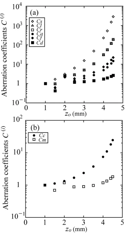
Before estimating the aberration due to the electro-static lenses, the dependence of the aberration coeffi-cients on the position of the object planes is investigated. The aberration coefficients referred to the object sideC(o)
(given by Eqs. (5) and (11)) are shown in Fig. 4 as a func-tion of the object planeszo. On the other hand, the
aber-ration coefficients referred to the image sideC(i)(given by
Eqs. (8) and (13)) are shown in Fig. 5 as a function of the object planeszo. In Fig. 5, the aberration coefficientsC(i)
are shown in a log scale. These aberration coefficients are normalized by the values atzo =1 mm. The mesh size is
0.1 mm.
Figures 4 and 5 show that the aberration coefficients C(i) vary with z
o larger than the aberration coefficients
C(o), except for the aberration coefficients of distortionC(i) d .
Forzo ≥ 2.5 mm, the aberration coefficientsC(i)increase
monotonically withzo.
The reasonC(o)andC(i)increase withzocan be
qual-itatively explained as follows: Aszo is closer to the
en-trance of the PG (or the negative ion source), the negative ion beams are affected significantly by the penetrating field in the PG. The penetrating field causes the negative ion beams to converge to the beam axis. Therefore, the nega-tive ion beams starting from the largerzocan pass the
loca-tions peripheral to the aperture, and then are more heavily influenced by the fringe field to aberration. This can be confirmed by comparing theh-trajectory forzo =1.0 mm
with that forzo=4.5 mm, as shown in Fig. 6.
Note that theh-trajectory starting fromzo = 1.0 mm
diverges after passing the location of z = zi. However,
this diverging trajectory does not contribute to aberration because the integration of aberration coefficients is per-formed in the range from z = zo toz = zi (see Eqs. (5)
and (11)).
The positions of the image planes zi are shown in
Fig. 4 Aberration coefficients referred to the object sideC(o)
given by Eqs. (5) and (11) in the main text. These aber-ration coefficients are normalized by the values atz=zo;
(a) geometrical aberration coefficients and (b) chromatic aberration coefficients.
zo becomes far from the entrance of the PG, the position
of the image planezibecomes far from the GRG exit. In
Refs. [6, 7], the negative ion beamlet profiles were mea-sured about 1.0 m downstream of the GRG. This corre-sponds tozi =1.25 m in the present model. From Fig. 7,
the value ofzi=1.25 m is obtained forzo=3.8 mm.
3.2
Dependence of aberration coe
ffi
cients on
mesh size
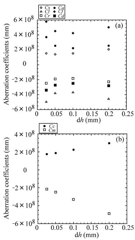
The aberration coefficients with the dimension of lengthc(i)(given by Eqs. (15) and (16)) are shown in Fig. 8
for zo = 4.0 mm. In the present calculation model, the
Fig. 5 Aberration coefficients referred to the image side C(i)
given by Eqs. (8) and (13) in the main text. These aber-ration coefficients are normalized by the values atz=zo;
(a) geometrical aberration coefficients and (b) chromatic aberration coefficients.
values ofφodepend on the mesh sizedh, even though the
position of the object planezois fixed. Thus, Fig. 8
com-pares the aberration coefficientsc(i)for four types of mesh
sizes: dh=0.025 mm (φo =16 V), 0.05 mm (φo =32 V),
0.1 mm (φo =64 V), and 0.2 mm (φo =128 V). The
mag-nifications M are almost constant for these four types of mesh sizes.
Fig. 6 Comparison ofh-trajectories forzo = 1.0 mm andzo =
4.5 mm.
Fig. 7 Position of the image planezias a function ofzo.
3.3
Contribution of electric field in the
extractor
/
accelerator to the aberration
coe
ffi
cients
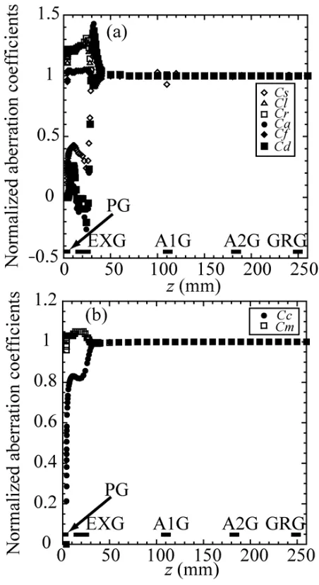
The contribution of the electric field at each zin the extractor/accelerator to the aberration coefficients is shown
z
zo
φ φo
F1h4+F2h3h+F3h2h2
dz− 1 32
φ φo
E1h4+E2h3h+E3h2h2+E5hh3
z zo
zi
zo
φ φo
F1h4+F2h3h+F3h2h2
dz− 1 32
φ φo
E1h4+E2h3h+E3h2h2+E5hh3
zi
zo
. (24)
Fig. 8 Aberration coefficients referred to the image side with the dimension of the lengthc(i)given by Eqs. (15) and (16) in
the main text. The position of the object plane is taken to bezo=4.0 mm. Comparison of aberration coefficients
c(i) for four types of mesh sizes: dh=0.025 mm (φ o =
16 V), 0.05 mm (φo = 32 V), 0.1 mm (φo = 64 V), and
0.2 mm (φo=128 V).
in Fig. 9. The mesh size and position of the object plane aredh = 0.025 mm andzo = 4.0 mm, respectively. The
vertical axis in Fig. 9 is defined such that the aberration coefficients referred to the object side atzin Eqs. (5) and (11) are normalized by those at the image planez=zi. For
The normalized aberration coefficients vary largely from the PG to the vicinity of the exit of the EXG, whereas they are almost constant from the A1G to the GRG. This indicates that the electrostatic lenses in the extractor con-tribute dominantly to the aberration, and the contributions
Fig. 9 Contribution of the electric field at eachzin the extrac-tor/accelerator to the aberration coefficients. The mesh size isdh=0.025 mm. The vertical axis is defined such that the aberration coefficients referred to the object side atzare normalized by those at the image planez=zi.
Table 2 Individual and total geometrical aberrations due to the electrostatic lenses.
dh Spherical Coma Coma Stigmatism Field Distortion Total
aberration curvatur
csui2u¯i cluiu¯iθ crui2θ¯i cau¯iθ2i cfuiθiθ¯ cdθ2iθ¯i
(mm) (mm) (mm) (mm) (mm) (mm) (mm) (mm)
0.025 19.1 −55.0 −27.5 36.6 57.0 −29.8 0.47
0.05 17.4 −43.9 −22.0 27.4 48.5 −27.0 0.36
0.1 19.0 −41.8 −20.9 23.2 44.0 −23.5 0.036
0.2 25.8 −52.9 −26.4 27.6 54.1 −27.9 0.16
from the electrostatic lenses in the accelerator are negligi-ble. This is due to the difference in strength of the conver-gent electrostatic lenses. As the negative ion beam velocity is much smaller in the extractor than in the accelerator, the space charge effect is larger in the extractor than in the ac-celerator. Therefore, to suppress the space charge effect, the electrostatic lenses are stronger in the extractor than in the accelerator.
3.4
Comparison of electrostatic lens
aberra-tions with negative ion beamlet profile
The aberration due to the electrostatic lenses are com-pared with the radii of the beam core and beam halo in Refs. [6, 7]. The aberrations for four cases of dh = 0.025 mm (φo = 16 V), 0.05 mm (φo = 32 V), 0.1 mm(φo =64 V), and 0.2 mm (φo =128 V) are estimated from the aberration coefficients in Fig. 8.
The overall aberration at the image plane is given as Δu(zi)=csui2u¯i+cluiu¯iθi+crui2θ¯i+cau¯iθ2i
+cfuiθiθ¯i+cdθ2iθ¯i−
ccui+cmθi
Δφ
φi
. (25) In the above equation,uiand ¯uicorrespond to the beam di-vergence angle of the beam core atz=zi. This divergence
angle of negative ion beamlet is taken to be 5 mrad. From Fig. 3,θiand ¯θi correspond to the beam divergence angle
of the beam core from the principal plane. The calcula-tion results show that the value ofθior ¯θiis approximately
4.5×10⁻³, regardless ofdh. The electrostatic potential at
the image planeφiis 406 keV.
The individual and total geometrical aberrations are shown in Table 2. In Refs. [6, 7], the measured 1/e radii for the beam core and halo are 5.8 mm (beam diver-gence angle: 6 mrad) and 11.5 mm (beam diverdiver-gence an-gle: 12 mrad), respectively. Each geometrical aberration is the same order as the radius of the beam halo. How-ever, the geometrical aberrations have positive or negative signs, and thereby cancel each other. The total geometrical aberrations are less than 1 mm. Thus, the total geometri-cal aberrations are much smaller than the radii of the beam core and halo.
Table 3 Individual and total geometrical aberrations due to the space charge effect.
αo Spherical Coma Stigmatism Field Distortion Total
aberration curvature
(mm) (mm) (mm) (mm) (mm) (mm)
0.1 −1.72×10⁵ 1.80×10⁵ −1.87×10⁵ −3.74×10⁵ 1.95×10⁵ −3.59×10⁵
0.2 −7.92×10⁵ 8.25×10⁵ −8.60×10⁵ −1.72×10⁵ 8.96×10⁵ −1.65×10⁶
Fig. 10 Chromatic aberrations as a function of the deviation of the initial kinetic energyeΔφ.
eΔφ. BeloweΔφ ≤100 eV, the chromatic aberrations are less than 2 mm, and negligible compared with the radii of the beam core and halo.
3.5
Geometrical aberrations due to space
charge e
ff
ect
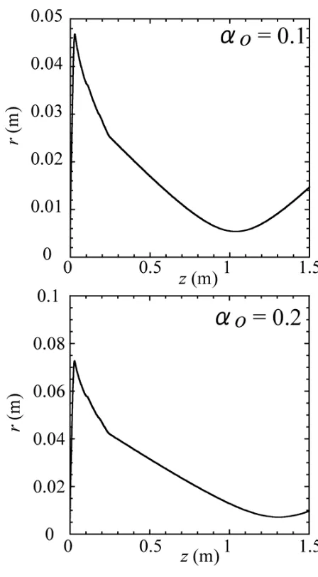
The geometrical aberrations due to the space charge effect are summarized in Table 3 fordh =0.1 mm. From Eq. (23), the H−beamlet trajectory orR(z) depends on the initial beamlet radiusRo, the incident angleαo at the
ob-ject plane, and the total currentI. In this calculation, Ro
is taken to be 7 mm. For the present calculation model, a realistic H−beamlet trajectory will become the minimum beam radius at the position where the negative ion profiles were measured in Refs. [6, 7] (z=1214 mm in the present model). The values ofαo=0.1 andαo=0.2 are taken
be-cause the corresponding H−beamlet trajectoriesR(z) be-come minimum aroundz = 1200 mm. The H− beamlet trajectoriesR(z) forαo = 0.1 andαo =0.2 are shown in
Fig. 11. The current density is 10 mA/cm2, thus, the total
current isπ×0.72cm2×10 mA/cm2=15.4 mA.
Comparing Tables 2 and 3 show that the geometrical aberrations increase drastically due to the space charge ef-fect. The total aberrations due to the space charge effect
Fig. 11 H−beamlet trajectories for the incident angles ofαo =
0.1 andαo = 0.2 with a negative ion current density of
10 mA/cm2.
range from 105to 106mm of order of magnitude, and are
4. Summary
The aberrations of the negative ion source/accelerator for neutral beam injector were theoretically estimated. The aberrations are considered to be caused by the electrostatic lenses, magnetic lenses, space charge effect, and shape of the beam-plasma boundary. In this study, the aberrations due to the electrostatic lenses and the space charge effect were investigated, and compared with the radii of the beam core and halo obtained in the H−beamlet profile measure-ments with the 400 keV negative ion accelerator. From this measurement, the 1/eradii of the beam core and beam halo were evaluated to be 5.8 and 11.5 mm, respectively. In the present calculation, the beam energy was taken to be 406 keV, and the electrostatic lenses were similar to those of the 400 keV negative ion accelerator. The aberration coefficients were numerically calculated using the eikonal method, which is conventionally used in electron optics.
The calculation results are summarized as follows: 1) The electrostatic lenses in the extractor dominantly
contribute to the aberration coefficients.
2) Based on the assumption that the divergence angle of the beam core is 5 mrad, the aberration due to the elec-trostatic lenses is less than a few millimeters, i.e., less than the radii of the beam core and halo. Therefore, the aberration due to the electrostatic lenses in the ex-tractor/accelerator is not the reason for the beam halo. 3) With a negative current density of 10 mA/cm2, the
ge-ometrical aberrations due to the space charge are es-timated to be from 105 to 106mm of order of
mag-nitude. Unlike the aberration from the electrostatic lenses, the geometrical aberration due to the space charge is much larger than the radii of the beam core and beam halo. Although the aperture radii of the grids are not taken into account in this estimation, the results indicate that the space charge effect is an im-portant factor in the aberration or beam halo in the negative ion accelerator.
Appendix. Eikonal Method
Let us consider the motion of a charged particle with an electric chargeeand massm. In the eikonal method, the variational functionFsatisfies
Δ
Fdz=0, (A1)
where F =
ˆ
φ1+x2+y2−ηAxx+Ayy+Az,
η=
e 2m, ˆ
φ=φ(1+εφ), ε= e
2mc2. (A2)
In Eq. (A2),cis the velocity of light. In the absence of a magnetic field, the magnetic vector potential is zero, i.e.,
Ax =Ay =Az =0. In the non-relativistic approximation, εis zero. Consider an optical system without a magnetic field, and the non-relativistic case. Moreover, the space charge effect is not taken into account.
First we deal with the geometrical aberration. From Eq. (A1), the Lagrange equation of motion is given as
d dz
∂F
∂¯u
−∂F∂¯
u =0, (A3-1)
d dz
∂F
∂u
−∂F∂u =0. (A3-2)
The characteristic functionF can be expanded as fol-lows:
F=F0+F2+F4+· · · , (A4)
F0=
φ,
F2=
√φ
2
uu¯−φ 4φ
,
F4=−
φ
1 128
φ2
−φ(4)φ
φ2
(uu)¯ 2+φ 16φ
uuu¯ u¯ +1
8
uu¯2
. (A5)
In Eq. (A5), F2 corresponds to the paraxial ray and
F4 corresponds to the aberration. When we neglect the
aberration termF4, Eq. (A3-1) is given as
d dz
∂(F
0+F2)
∂¯u
−∂(F0+F2)
∂¯u =0. (A6) By substituting Eq. (A5) into (A6), we obtain
u+ φ 2φu+
φ
4φu=0. (A7)
Equation (A7) is the paraxial equation, and the solu-tion corresponds to the paraxial rayuG.
In estimating the aberration, we should take F4 into
account for Eq. (A3-1): d
dz
∂(F
0+F2+F4)
∂¯u
−∂(F0+F2+F4)
∂¯u =0. (A8) Equation (A8) can be written as
d dz
∂F
2
∂¯u
−∂F2
∂¯u = ∂F4
∂¯u − d dz
∂F
4
∂¯u
. (A9)
The solution of Eq. (A9) will be written asu=uG+u3,
whereuGandu3 are the paraxial rayuGand geometrical
aberration, respectively. Note that u3 is the third order
term. By substitutingu = uG+u3 into the left side, we
obtain d dz
∂F
2
∂¯u
−∂F2
∂¯u =
√φ
2
(uG+u3)+
φ
2φ(uG+u3)
+φ4φ(uG+u3)
SinceuGis the solution of the paraxial equation (A7),
Eq. (A10) can be transformed into d dz ∂F 2 ∂¯u
−∂F2
∂¯u =
√φ
2
u3 + φ 2φu3+
φ 4φu3
.
(A11) On the other hand, let us define the right side of Eq. (A9) as
W =Wu,u,¯ u,u¯,u,u¯=∂F4 ∂¯u −
d dz ∂F 4 ∂¯u . (A12) The right side of Eq. (A9)W(u,u,¯ u,u¯u,u¯) can be expanded in Taylor’s series:
Wu,u,¯ u,u¯,u,u¯ =WuG,u¯G,uG,u¯G,uG,u¯G
+ ∂W∂¯ u
Gu¯3+
∂W ∂u G
u3
+ ∂W∂¯ u
Gu¯3+ ∂W ∂uGu3+
∂W ∂¯u
Gu¯3 + ∂W ∂uGu3.
(A13) In Eq. (A11), ∂W∂¯
u
G, ∂W∂u
G
, ∂W∂¯ u
G, ∂W∂u
G
, ∂¯∂W u
G, ∂W
∂uG denote ∂W
∂¯u
u¯=u¯
G
, ∂W ∂uu=uG
, ∂W ∂¯u
u¯=u¯G
, ∂W ∂uu=uG
, ∂W
∂¯u
u¯=u¯G
, ∂W ∂uu=uG
, respectively. In the third or-der approximation of the aberration, the terms ∂W
∂¯u
Gu¯3,
∂W ∂uG
u3,
∂W ∂¯u
Gu¯3, ∂W ∂uGu3,
∂W ∂¯u
Gu¯3, ∂W
∂uGu3 can be
negligible, sinceu3is the third order term. Thus, we obtain
Wu,u,¯ u,u¯,u,u¯=WuG,u¯G,uG,u¯G,uG,u¯G
. (A14) Note that from Eq. (A14), mathematically,u, ¯u,u, ¯u, u, ¯u on the right side of Eqs. (A9) or (A12) are equiv-alently replaced withuG, ¯uG, uG, ¯uG, uG, ¯uG. Thus, we
define F4G as F4G = F4
uG,u¯G,uG,u¯G
, and in the third approximation of the aberration, we obtain
Wu,u,¯ u,u¯,u,u¯= ∂F4G ∂¯uG
−d
dz
∂F
4G
∂¯uG
. (A15)
From Eqs. (A11) and (A15), the ray equation for the aberration is given as
√φ
2
u3 + φ 2φu3+
φ 4φu3
=∂F4G
∂¯uG −
d dz
∂F
4G
∂¯uG
.
(A16) We set the solution of Eq. (A16) as
u3=αg+βh. (A17)
Moreover, we add the condition of
αg+βh=0. (A18)
The initial condition for the aberration is set at u3(zo) = u3(zo) = 0. By applying Lagrange’s method of
undetermined multipliers to Eq. (A17), we obtain α=
2 φ0
∂F4G
∂¯uG h
z
zo
− √2φ
0
z
zo
∂F
4G
∂u¯G
h+∂F∂¯4G uG h
dz,
β=
−φ2
0
∂F4G
∂u¯G g
z
zo
+ √2φ
0
z
zo
∂F
4G
∂¯uG
g+∂F4G
∂¯uG g dz.
(A19) The initial condition for the paraxial ray is set to be uG(zo) = uo, uG(zo) = uo. The paraxial ray can be
ex-pressed as
uG(z)=uog(z)+uoh(z). (A20)
Thus, we obtain
uG(z)=uog(z)+uoh(z),
¯
uG(z)=u¯og(z)+u¯oh(z),
¯
uG(z)=u¯og(z)+u¯oh(z). (A21)
From Eq. (A21), we can obtain the following rela-tions:
∂F4G
∂¯uo
= ∂F4G
∂¯uG
h+∂F∂¯4G uG h
,
∂F4G
∂¯uo =
∂F4G
∂¯uG
g+∂F4G
∂¯uG g
. (A22)
By substituting Eq. (A22) into Eq. (A19), we obtain α=
2 φo
∂F4G
∂¯uG h
z
zo
− √2φ
o
∂ ∂¯uo
z
zo
F4Gdz,
β=
−φ2
o
∂F4G
∂¯uG g
z
zo
+ √2φ
o
∂ ∂¯uo
z
zo
F4Gdz. (A23)
The values ofg(z) andh(z) at the image planez =zi
are given byg(zi)=M,h(zi)=0 (see Fig. 3). Thus, with
Eq. (A17), the aberration atz=ziis expressed as
u3(zi)=α(zi)g(zi)+β(zi)h(zi)=Mα(zi). (A24)
By replacingu, ¯u,u, ¯uin the termF4with the
parax-ial solutions uG, ¯uG, uG, ¯uG, and substituting Eqs. (A20)
and (A21) into Eq. (A23), we obtain α=
2 φo
∂F4G
∂¯uG h
z
zo
+C(o)s uo2u¯o2+Cl(o)uou¯ouo
+C(o)r uo2u¯o+Ca(o)u2ou¯o+C (o)
f uou¯ouo+C (o) d u
2 ou¯o,
(A25) where the coefficients ofC(o)s ,Cl(o),C
(o)
r ,C(o)a ,Cf(o),C (o) d are
given as follows: Cs(o)=
z zo φ φo 1 32
φ2
−φ(4)φ
φ2
h4
+φ4φh2h2+1 2h
4
1 2C
(o) l =C
(o) r =
z
zo
φ
φo
1 32
φ2−φ(4)φ
φ2
gh3
+φ8φ(gh)hh+1 2g
h3
dz,
C(o)a =
z
zo
φ φo
1 32
φ2
−φ(4)φ
φ2
g2h2
+φ4φgghh+1 2g
2h2
dz,
C(o)f =
z
zo
φ φo
1 32
φ2
−φ(4)φ
φ2
g2h2
+φ8φ(gh+gh)2+g2h2
dz,
C(o)d =
z
zo
φ φo
1 32
φ2
−φ(4)φ
φ2
g3h
+φ8φgg(gh)+1 2g
3hdz. (A26)
The first term on the right side of Eq. (A25) becomes zero becauseh(zo) =h(zi)=0. Therefore, the aberration
is given by u3(zi)=M
C(o)s uo2u¯o+C (o)
l uou¯ouo+C(o)r uo2u¯o
+C(o)a u2ou¯o+C (o)
f uou¯ouo+C (o) d u
2 ou¯o
. (A27) The chromatic aberrationuccan be calculated with a
similar procedure, and is given by Eqs. (10) and (11) in the main text.
[1] T. Inoueet al., Rev. Sci. Instrum.71, 744 (2000).
[2] ITER EDA Final Design Report, ITER technical basis, Plant Description Document (PDD), G A0 FDR 1 01-07-13 R1.0, IAEA EDA documentation No. 24, 2002. [3] T. Inoueet al., Rev. Sci. Instrum.75, 1819 (2004). [4] M. Taniguchiet al., Rev. Sci. Instrum.77, 03A514 (2006). [5] A.J.T. Holmes and M.P.S. Nightingale, Rev. Sci. Instrum.
57, 2402 (1986).
[6] K. Miyamoto et al., in Proceeding of the joint meeting of the 7th International Symposium on the Production and Neutralization of Negative Ions and Beams and 6th Euro-pean Workshop on the Production and Application of Light Negative Ions (Upton, New York, Oct. 23∼27, 1995), AIP Conference Proceedings 380 (1996) p. 390.
[7] K. Miyamotoet al., in Proceedings of the 17th IEEE/NPSS Symposium on Fusion Engineering (San Diego, California, Oct. 6∼10, 1997), vols.1 and 2 (1998) p. 1067.
[8] R.S. Hemsworthet al., Rev. Sci. Instrum.67, 1120 (1996).
[9] P.W. Hawkes, Magnetic Electron Lenses, Chapt. 1
(Springer Verlag, 1982).
[10] F.H. Read, J. Phys. E2, 165 (1969). [11] F.H. Read, J. Phys. E3, 127 (1970). [12] E. Munro, Optik39, 450 (1974).
[13] A. Renau and D.W.O. Heddle, J. Phys. E19, 288 (1986). [14] S. Naganachiet al., Rev. Sci. Instrum.67, 2351 (1996). [15] T. Tang, J. Orloffand L. Wang, J. Vac. Sci. Technol. B14,
80 (1996).
[16] K. Sakaguchi and T. Sekine, J. Vac. Sci. Technol. B 16, 2462 (1998).
[17] K. Kanaya, H. Kawakatsu and H. Yamazaki, Br. J. Appl. Phys.16, 991 (1965).
[18] W. Glaser, Elektronen und Ionenoptik. Handbuch der Physik33, 123 (1956).
[19] K. Ura, Electron and Ion Beam Optics, Chapt. 15
(Kyouritsu Shuppan CO., LTD., 1994) [in Japanese]. [20] S. Takashima,Basis of Theory and Simulation for Electron
Optics[JEOL textbook in Japanese, unpublished]. [21] P.W. Hawkes, Adv. Electronics and Electron Physics,
Suppl.7(Academic Press Inc., June, 1970).
[22] M. Kuriyamaet al., Fusion Sci. Technol.42, 410 (2002). [23] Y. Okumuraet al., Rev. Sci. Instrum.67, 1018 (1996). [24] K. Miyamotoet al., in Proceedings of the 18th Symposium
on Fusion Technology (Karlsruhe, 1994), Elsevier, Amster-dam, vol.1 (1995) p.625.
[25] M. Hanadaet al., Rev. Sci. Instrum.69, 947 (1998). [26] T. Morishitaet al., Rev. Sci. Instrum.73, 1064 (2002). [27] M. Hanadaet al., Rev. Sci. Instrum.77, 03A515 (2006). [28] A. Hatayama, Rev. Sci. Instrum.79, 02B901 (2008). [29] R. Becker, Rev. Sci. Instrum.67, 1132 (1996). [30] O.I. Seman, Radiotech. Electron.3, 402, 1702 (1958). [31] P.W. Hawkes, Optik24, 252 (1966/67).