Modeling and Analyzing Hydrocyclone Performances

Modeling and Analyzing Hydrocyclone Performances

Samaeili, Milad

Department of Chemical Engineering, Islamic Azad University, Mahshahr Branch, Mahshahr, I.R. IRAN

Hashemi, Jalaleddin*

Department of Mechanical Engineering, Petroleum University of Technology (PUT), Ahvaz, I.R. IRAN

Sabeti, Morteza

Department of Chemical Engineering, Isfahan University of Technology, Isfahan, I.R. IRAN

Sharifi, Khashayar

Iran Research Institute of Petroleum Industry (RIPI), Tehran, I.R. IRAN

ABSTRACT: Hydrocyclones have been used as an operational tool to separate liquids from solids in different industries for more than 50 years. Considering the importance of this issue, many experimental and numerical attempts have been made to estimate the performance of this tool regarding the resulting pressure drop and the separation efficiency (particles separation limit diameter). Most of the numerical studies for simulating the fluid flow pattern inside Hydrocyclones have been conducted using the ‘’Fluent’’ commercial software. The other alternative for this evaluation is the application of CFD in COMSOL Multiphysics. This work is mainly focused on studying the effect of entering tangent velocity and also determining the flow pattern by CFD simulation in the powerful COMSOL Multiphysics software. Thereafter, correlations proposed by a number of authors are compared with experimental data to evaluate their performances. Among them, the correlations suggested by Barth and Koch-Lich showed acceptable accordance with reference data and thus were chosen for sensitivity analysis. Based on the results, three geometrical parameters of the hydrocyclone body have considerable effects on the separation efficiency. The findings revealed that decreasing the outlet diameter and the inlet width result in increasing the efficiency of hydrocyclone while enlarging the body diameter has negative effects on it. Furthermore, the cyclone efficiency is enhanced as the density difference between fluid and solid and the input velocity becomes larger.

KEYWORDS: Hydrocyclone; CFD simulation; Mathematical model; Hydrocyclone performance field flow and pressure drop; Sensitivity analysis.

INTRODUCTION

Hydrocyclone is a cylindrical-conical device. Those specifically designed for liquids are called hydrocyclone

or hydraulic cyclone. The separation inside a hydrocyclone is based on centrifugal sedimentation, where the suspended

*To whom correspondence should be addressed. +E-mail: [email protected]

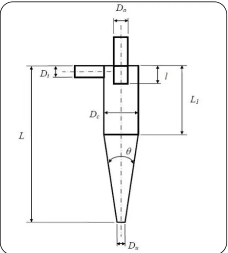
Fig. 1: A scheme of hydrocyclone configuration.

the particle is exposed to the centrifugal acceleration that leads to their separation from the fluid carrying them [1]. Although the centrifugal force is created inside a cyclone, no moving parts exist in it and the required vortex flow is formed by the fluid itself. Fig. 1 illustrates the cross-section of a hydrocyclone with a common design.

As indicated by the figure, a hydrocyclone is formed by a cylinder which is connected to its lower part. Particles suspended in the liquid enter the hydrocyclone tangent to its entrance and due to this tangent motion of the fluid, a vortex flow is formed inside the hydrocyclone. A portion of liquid that carries fine particles is ejected through a cylindrical outlet placed at the top of the hydrocyclone. This outlet is known as the overflow pipe or vortex finder. The remaining liquid which bears larger particles is ejected through the cylindrical outlet at the bottom of the cone. This outlet is called spigot or underflow orifice. As can be seen, various parameters affect the performance of hydrocyclones. To know the performance of hydrocyclones, engineers are able to use a lot of mathematical models to simulate the potential of the hydrocyclones. However, there exist totally two main types of mathematical models that give a helping hand to the engineers to obviate their obstacles [2]. Both of the methods are described in the proceedings.

To recognize the performance of a hydrocyclone, including particle sizes selectivity, efficiency, and mass flow in the overflow and spigot parts, investigators can take the advantage of semi-analytical models. The customary approaches for this type of the models are implementing the residence time and equilibrium orbit theorems [3-4]. These models, usually utilized for hydrocyclone sizing, are both explained in the theory section of this manuscript in detail.

by the hydrocyclone due to the high rotational velocity of the fluids, an air core phase appears in the center of the equipment, which totally increases the complexity in conceiving and scrutinizing the performance of the hydrocyclone from a mathematical point of view. Some worked on other turbulence's model such as Reynolds stress model years later. The results show that RSM's outcome is more promising than previous approaches [11-13]. Xu et al. [14] classified numerical methods for modeling a hydrocyclone. They claimed that of RNG, k-ԑ, RSM and LES and so on [15], the LES and RSM have more potential to produce results to be much closer to experimental data.

The other aspect of hydrocyclone simulation to be considered is an accurate visualization of the motion of dispersed and continuous phases inside hydrocyclones. Several researchers to deal with momentum and continuity equations employed Eulerian approach [16-18], and some other took the advantage of Lagrangian approach [19-20] to predict the path of each individual particle when entering hydrocyclone medium.

Ghadirian et al. [21] took the advantage of the LED method to improve the numerical study was done by Delgadillo and Rajamani [9]. Exploiting Ansys 12 Fluid Dynamic, they simulated two hydrocyclones with different geometries. Their results included the measuring pressure inside the hydrocyclones and determining velocities as well as separation efficiencies. Finally, the authors indicated that their mathematical model could predict better due to its LED turbulent model and ts proper domain discretization they hired in their research. It was admitted by Hsu et al. [22] that a study into the computational fluid dynamic of a hydrocyclone needs a meticulous simulation to show how a certain change of the boundary conditions can influence the separation process.

This survey mainly investigates the fluid velocity distribution and the performance of separating solid particles in the mixture entering the hydrocyclone by simulation and mathematical modeling. Thus, a study is presented for evaluating and studying the flow profile of liquid-solid inside the hydrocyclone using the commercial COMSOL Multiphysics 3.5. Then, to evaluate the hydrocyclone efficiency at different conditions using determined correlations semi-analytical models are conducted. Next, the results of the simulation

and hydrocyclone modeling are presented; in the end, regarding the results, the available models are analyzed and a proper conclusion based on the survey outcomes is arisen.

THEORETICAL SECTION

The governing equations for sketching flow patterns of fluid inside hydrocyclone are firstly studied by numerical modeling and then, the well-known correlations in this field which are based on physical features of hydrocyclones and fluids are scrutinized in the next other parts of the following section so as for the overflow and under flow properties to be estimated.

Numerical modeling

The details about simulation procedure such as determining the geometry of hydrocyclone, materials, boundary conditions, gridding, solution method and analysis after the process by COMSOL Multiphysics 3.5 are discussed in this section. To simulate the dynamic of fluid the steady Navier-Stokes, k-ε turbulence model, as well as a dispersion equation, are employed. These relations are shown in following forms. According to chemical engineering module of COMSOL Multiphysics, the only sturdy branch that helps us to find this model is mixture model. This model provides researchers with enough potential to compute flow for a liquid-solid mixture accurately.

 





        (1)













 

 

w .u 0

   (3)





. u 0

    (4)

Where u, p, Cd, uslip,τGm, ρs and ρw represent mixture

velocity, the pressure of the system, mass fraction of the solid phase, slippage velocity between the dispersed and the main fluid, the sum of viscous and turbulent stress, the solid and the fluid density, in the same order. In addition, Фs is volume fraction of the solid (dispersed phase)

and Dmn shows the solid dispersion coefficient

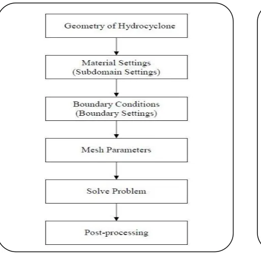
Fig. 2: The overall trend in hydrocyclone simulation by COMSOL Multiphysics 3.5.

Fig. 3: A scheme of the equilibrium orbit theorem background.

 

k

C k

u. k .   k

     _ _   

  

  (5)

 

2 2

k

0. 5 C _ u 



 

k

C k

u. .   

      _ _   

  

 

(6)

 

1 2

0. 5 C C k u C

k

  



  

Where for the k-ε turbulence model, k is the turbulent kinetic energy and ε represents the turbulent dissipation rate. Moreover, other parameters have a constant value that should be estimated depending upon defined conditions in the physical features of the problem. In this study, the values ordered by COMSOL Multiphysics are used.

The following flowchart in Fig. 2 describes the trend from the beginning and program operation to find the results.

Semi-analytical models

To evaluate the configuration of a hydrocyclone, it is necessary to model the fluid velocity distribution inside it. This has been the motivation for several researchers and

authors, leading to the valuable findings available in the literature for hydrocyclone flow pattern determination. Basically, there are two distinct concepts for hydrocyclone performance evaluation based on which the hydrocyclone is modeled. These two theories are known as ‘’Equilibrium orbit’’ and ‘’Residence time’’. In proceedings, fundamental equations that own fewer complexities are presented to describe the concepts of these theories [3-4].

The equilibrium orbit theorem

Fig. 3 describes the background concept of the equilibrium orbit theorem. In this model, researchers consider an indiscrete Cylindrical Surface (CS) from top to bottom of the cyclone. This theorem is based on the force balance on the particle rotating around the cylindrical surface. The radius of this surface is equal to half of the vortex leading diameter, Rx = 1/2Dx.

In this balance, the external centrifugal force is balanced by the internal drag force due to fluid resistance. In the centrifugal force, force is proportional to x3_{, while}

by a lot of researchers, this size is the basis for evaluating and modeling Hydrocyclones, for it could be assumed

no particle bigger (smaller) than can enter the overflow (spigot) [23].

Particles for which these two opposing forces are equal will always rotate in the CS region and are known as particles with the separation limit diameter (or cut

size), . Indeed, they have equal chances (50-50) of exiting the cyclone through either the spigot or the vortex finder. The separation limit diameter can be obtained by the below equation after simplifying the equations of radial and tangent velocities and also the centrifugal and drag forces exerted to the particles [24].

rC S x

5 0 2

C S

v D

x 9

v_

 

 (7)

Residence time theorem

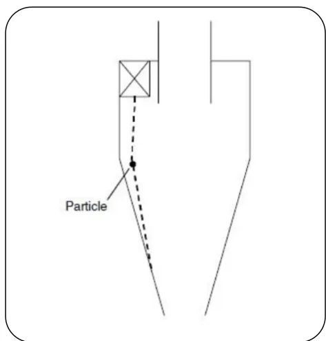
Fig. 4 shows another approach to the modeling. Here, the movement of the solid particle with regard to the cyclone wall is of particular interest and the velocity of fluid entering the cyclone is neglected. In fact, this theory deals with the question that: after entering the cyclone, will the particle have enough time to reach the wall and settle in the spigot before reaching the end of the cyclone?

Rosin et al. (cited in [25]) were the first researchers to calculate the separation limit diameter by this theory. To do this, they compared the time required for the particle to reach the cyclone wall at any radius with the time just before it reaches the cyclone bottom. Thus, the finest particle that would traverse the radial distance after entering the cyclone (the whole entrance width) before reaching the bottom was called the particle with the separation limit diameter (or cut size), x50.

5 0

s i n p

9b x

N v ( )

 

   (8)

To solve this equation, it is necessary to have the value of Ns. In 2001, Zenz [26] proposed a graph of Ns

versus the input velocity. The equation is as follows.

i n

0.0066v s

N 6.1(1 e  ) (9)

Fig. 4: A scheme of the residence time theorem background.

Empirical model

There are some available empirical models with industrial applications of which one of the most important ones is Plitt’s [27]. Plitt performed his experiments in hydrocyclones with 1.25 in 6 in. dimensions. Besides his own experiments, he enjoyed the results of Lynch and Rao’s work (cited in [28]). In fact, he gathered a total of 300 experiment types on several hydrocyclones. In addition to dimensional variables such as the entrance diameter, vortex finder, and the spigot, this researcher investigated the height of the vortex finder and the hydrocyclone body diameter. Moreover, he considered the variables of input and output. In the end, he offered the modeling relationships by linear regression. In this model, knowing all hydrocyclone dimensions as well as the other particles distribution range, it is possible to calculate the pressure drop, particle separation limit diameter, and the flow fraction. Below equations are used to find the hydrocyclone conditions.

Calculating the separation limit diameter,

0. 063cv

0. 46 0. 6 1. 21

i x

50 1 0. 71 0. 38 0. 45

p f

5 0 . 5D D D e

x C

B h Q ( )

 

 

 

   

 

(10)

Where C1 is the correction factor used for exact

Pressure drop along the hydrocyclone,

0. 0055cv

1. 78

2 0. 37 0. 94 0. 28 2 2 0. 87

i x

1 . 8 8Q e

p C

D D h (B D )

            (11)

In which C2 is the correction factor for obtaining

the pressure drop in the hydrocyclone.

The value of input rate with respect to the spigot Rv

is equal to,

v

S R

S 1



 (12)

Where S stands for the flow fraction (vortex flow to feed flow) and is equal to,

v

3 . 3 1

(0 .0 0 5 4c ) 0 .5 4 2 2 0 .3 6

x x

3 0 .2 4 1 .1 1

B

1. 9 h (B D ) e

D S C H D  _{ }        _{ }   _        (13)

In which C3 is the correction factor for exact

determination of the hydrocyclone flow fraction. Also, in the above equation, H shows the pressure drop per meters of fluid.

To describe the slope of the efficiency diagram, m is defined as follows,

0. 15 2 v

D h ( 1. 58R )

Q

4

m C 1. 94e

 _{ } 

 _ _ 

 _{ } 

 

  (14)

Where Q is the hydrocyclone input flow rate and C4 is

the correction factor applied to the slope of the hydrocyclone performance diagram.

Finally, Plitt [27] proposed the following relation for calculating the performance coefficient.

m i 50

x 0 . 6 9 3

x

i

y 1 e

 _{ } 

 _ _ 

 _{ } 

 

  (15)

Plitt’s model is capable of yielding the desired results without adjusting the constant coefficients. This is actually the privilege of his model over other ones. Of course, neglecting the particle size distribution function is considered as its deficit compared to other empirical models [27].

The grade efficiency of a hydrocyclone defined by Eq. (16) [23] depends on several factors such as hydrocyclone dimensions, particles density, physical

properties of the fluid and input and output conditions. This section is aimed at studying different models based on equilibrium orbit and residence time theories. Meanwhile, seven famous models are compared here and the best one is chosen for further analysis. It should be noted that in this paper, coefficients of Plitt’s model are updated by optimization rules regarding the input conditions so as to obtain more eligible results.

Mass flow in size grade in spigot (kg / s) G.E

Mass flow in size grade in feed (kg / s)

 (16)

RESULTS AND DISCUSSION

To analyze the flow pattern of the fluid as well as the slippage velocity of particles inside hydrocyclone from the qualitative and quantitative point of view, the estimated results from the present numerical modeling and semi-analytical correlations are compared with the experimental data extracted from Ipate’s work [29]. The fluid and solid particles used in this simulation have the characteristics presented in Table 1.

All boundary conditions in a hydrocyclone of some levels with the feed, cyclone wall, spigot and the vortex finder can be divided into four classes which are alluded to in Table 2.

Numerical modeling

A typical geometry sketched by COMSOL toolbox is shown in Fig. 6. The body of hydrocyclone volume is set to the specified characteristic defined in Table 1 and Table 2 also is employed to clarify the surface of hydrocyclone as well as the overflow and underflow surfaces as the boundaries of the geometry. Unstructured Tetrahedral and Hexahedral grids are designed for this study as the values of aspect ratio and skewness of the cells to be set on desirable quantities almost. To have accurate results each of the different parts of hydrocyclone such as cylindrical body or vortex finder, are meshed separately. A grid independence investigation is conducted here with the help of modeling with various mesh densities, and finally, the 55000-elements as an optimal choice for computation is selected to proceed the next steps.

Table 1: Physical properties of materials used in simulation [29].

Forming materials amount

Liquid density (kg/m3₎

998

Solid particles density (kg/m3₎

2700

Fluid viscosity (Pa.s) 0.001

Other particles under study (m) 5-400

Table 2: Boundary conditions used in hydrocyclone simulation.

Defined boundaries parameter amount

Hydrocyclone wall velocity 0(no slippage)

Feed velocity 1.28 m/s

Vortex finder pressure 0 KPa

spigot pressure 0 KPa

Fig. 5: Comparison between outputs arisen from COMSOL Multiphysics and experimental data extracted from [29].

the set of measures taken to study and analyze the proposed model after problem-solving is called post-processing analysis. This is the final step done in the present study. To do so, several features available in COMSOL tools such as contour plot are exploited, some of which are presented in the next parts.

One of the important way to perceive the potential of a numerical model is to compare the results of the model to experimental data. In order to validate the present model coming from COMSOL, the outcomes are compared with Ipate’s work [29]. The comparison to be considered are exhibited in Fig. 5. As shown in this figure, grade efficiency for a wide range of particle sizes is calculated and then sketched using the COMSOL

toolbox. At the beginning (particle size ranging from 1 to 70μm), there are differences between the experimental and numerical data. Although there exist some reasons, such as ignoring air core inside hydrocyclone, that explains why there are discrepancies between these two results, from an academic point of view, it can be taken as a fairly successful model to proceed and study more about various important factors affecting the performance of the hydrocyclone.

Static pressure

Although COMSOL is confronted with a number of limitations in hydrocyclone simulation, the results of static pressure distribution implicitly give evidence on the formation of a cylindrical surface (CS) in the hydrocyclone. It is obvious from Fig. 6 that the minimum or even negative values of hydrostatic pressure is placed in a region in the center of cyclone axis which in turn reveals the existence of a cylindrical surface, CS.

At any height of the axis column, the static pressure has its maximum value near the wall and decreases toward the center. In addition to that, the static pressure decreases from top to bottom (vortex finder to spigot). Hence, suspended particles near the hydrocyclone wall are drawn down with a rotational motion. Moreover, the pressure drop in the center of hydrocyclone decreases in such a way that particles close to CS region can vertically or rotationally move upward and get out through the vortex finder.

Particle diameter (1e-6m)

0 100 200 300 400 500

Gra

d

e

ef

fi

ci

en

cy

1.2

1

0.8

0.6

0.4

0.2

Fig. 6: Pressure distribution in the x-y plane at different heights z from the plane.

Fig. 7: Axial velocity distribution with a counter view of velocity in vertical cross-section.

Axial velocity

Fig. 7 can help understand one of the most important characteristics of the axial motion of the fluid inside a hydrocyclone. As can be seen in the figure, the axial velocity is negative near the cyclone body i.e. it is downward, while the velocity in the cyclone center is positive. The intersection of these two opposite velocities is where the axial velocity is zero and is known as Locus of Zero Vertical Velocity (LZVV) [5, 30-31]. LZVV can be estimated with the help of Fig. 8. It should be noted that particles passing along LZVV boundary can be approximately considered as particles of separation limit diameter. Since particles orbiting at radial distances more than the LZVV will fall down toward spigot while those that are inside the LZVV area will go into overflow [23]. Thus, the LZVV flow path can give another statement for defining the hydrocyclone performance in solid particles separation and using LZVV area it is possible to estimate the cut size of the particles in the hydrocyclone [23]. Moreover, the value of axial velocity has a vital role in determining LZVV boundary inside hydrocyclone and the residence time of particles [5, 30-31]. It was asserted that an increase in the hydrocyclone’s inlet velocity results in an increase for downward (outside of LZVV interface) and upward (inside of LZVV interface) flows. Thus, it is expected that the required time for a part of the

mixture to wait inside hydrocyclone decreases as the inlet velocity increases. So, increasing the vertical velocity reduces the residence time. Regarding the residence time theorem mentioned in upper sections of this manuscript, it is obvious that a reduction of residence time culminates to a reduction for the particle cut size. Therefore, an increase in the inlet velocity causes the cut size diameter decreases. This phenomenon is also admitted by semi-analytical models (See Effect of Input Velocity in the proceedings).

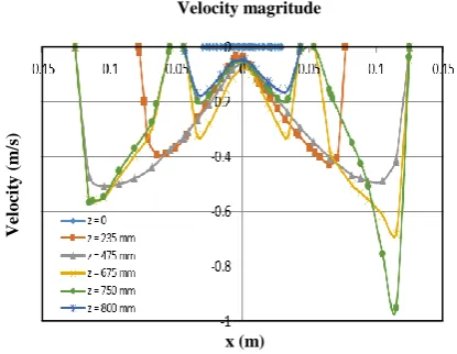
Tangent velocity

Fig. 8: A cross-sectional area inside the hydrocyclone that shows the distribution of axial velocity as well as the boundary inside the hydrocyclone that there exists a zero axial velocity (LZVV).

Fig. 9: Tangent velocity counter distribution on the x-z plane.

Particles slippage velocity

So far, it has been clarified that upon the entrance of fluid in the hydrocyclone, the centrifugal force is exerted on the particles due to the rotational movement of the fluid, making them move toward the cyclone body. Fig. 10 shows the value of the difference between fluid and particles velocity (particles slippage velocity) as directed vectors in different cross-sections. The presented vectors in any cross-section point outward. This reveals that at any height, an external force is being exerted on the particles. Besides, Fig. 10 (b) depicts that the particles

slippage velocity decreases from top to bottom, for the maximum value of tangential velocity at each height reduces with a decrease in axial height, then, at lower portion of the hydrocyclone height there are relatively lower centrifugal forces to develop huge slippage velocities for the solid particles.

Recovery coefficient estimation

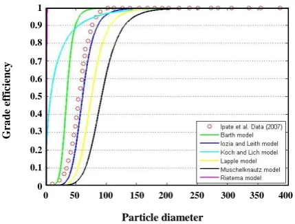
Fig. 11 represents the results of the comparison made between the models proposed by Bart (cited at [32]) (equilibrium orbit), Iozia and Leith [33] (residence time), Koch and Lich [34] (residence time), Lapple (cited at [35]), Muschelknautz (cited at [36]) (equilibrium orbit), Rietema [37] (residence time) and the data given by Ipate and Căsăndroiu [29] on the calculated value.

The model offered by Iozia and Leith gives an excellent estimation compared to the data at mentioned conditions. Models of Lapple and Muschelknautz give a relatively smaller estimation of the grade efficiency, while Barth’s and Rietema’s models suggest larger values at a certain particle diameter. The model presented by Koch and Lich give larger estimates for finer particles, while this becomes vice versa for particles of greater diameter.

Due to a shortage of space here, it is not possible to investigate all aforementioned models. Hence, the two famous models suggested by Barth and Koch-Lich are chosen due to their significant operational efficiency to study the effect of various parameters on hydrocyclone performance from the aspects of equilibrium orbit and residence time theories. In proceedings, they are analyzed.

The effect of particles density on efficiency

The difference between the densities of solid and

liquid





the cyclone performance. The efficiency coefficients at various density scales in the two Barth and Koch-Lich theories are demonstrated. As can be seen, a larger particle density tends to create a greater centrifugal force which itself results in the reduction of separation limit diameter and finally increases grade efficiency. Moreover, the efficiency coefficient plot versus particles diameter will have a greater slope if the density difference enlarges. It should be also noted that this difference plays a more significant role in the efficiency of gas-solid cyclones than in liquid-solid cyclones. x (m)

V

el

o

ci

ty

(

m

/s)

Fig. 10: Particles slippage velocity distribution at different heights. (A): normal slippage velocity distribution, (B): slippage velocity distribution.

Fig. 11: Comparison between data presented by Ipate and Căsăndroiu [29] and estimation of grade efficiency with respect to particle size using the 6 models.

Fig. 12: Effect of particles density on efficiency coefficient using Barth and Koch-Lich models.

That is because the gas densities are much smaller than liquids’ by some orders.

Effect of input velocity

The velocity of feed fluid, i, is an influential

parameter in cyclone design for obtaining an appropriate separation performance. The velocity of the entering fluid can be found by dividing the value of input flow rate to the input cross-section area. A large flow rate will result in a high input velocity. The separation diameter is proportional to the inverse of input velocity squared. Fig. 13 indicates the effect of input velocity on hydrocyclone

performance. It shows that at same particle sizes and certain cyclone geometries, a larger input velocity yields greater slopes on the grade efficiency plot.

However, it can be seen that too large velocities will have inverse effects on cyclone performance since turbulency, saltation and re-entrainment occur at such velocities. Considering these severe effects, an input velocity of 18 m/s is known as the optimal input velocity [38].

Effect of entrance width

As the width of hydrocyclone entrance, b, becomes larger, the formed vortex expands more and becomes weaker, Particle diameter

0 50 100 150 200 250 300 350 400

Gra

d

e

ef

fi

ci

en

cy

1

0.9

0.8

0.7

0.6

0.5

0.4

0.3

0.2

0.1

0

Particle diameter

0 20 40 60 80 100 120 140 160 180 200

Gra

d

e

ef

fi

ci

en

cy

1

0.9

0.8

0.7

0.6

0.5

0.4

0.3

0.2

0.1

Fig. 13: Effect of input velocity on cyclone efficiency. Fig. 14: Effect of entrance width on cyclone efficiency.

Fig. 15: Appropriate and inappropriate pattern of fluid’s rotational flow at different entrance widths.

which finally reduces the efficiency. Fig. 14 indicates the impact of cyclone width enlargement on grade efficiency reduction. A weak vortex yields fewer rotations inside the cyclone and leads to separation efficiency reduction. Fig. 15 represents the flow patterns at two different entrance widths as well as the corresponding disorder made in hydrocyclone performance due to excessive increasing of the entrance width. Coker suggested that the best width must be less than (D-De)/2 [39].

Body diameter and hydrocyclone vortex leader diameter It is essential to consider the effect of cyclone diameter on separation limit diameter at operational conditions. Generally, it has been indicated that the separation limit diameter is proportional to the diameter of hydrocyclone body and vortex finder. For investigation and comparison,

body diameters of 0.2 m, 0.25 m and 0.3 m were selected and considered in Barth and Koch-Lich models. Fig. 16 gives the result of this comparison at an input velocity of 1.28 m/s. It suggests that increasing the hydrocyclone body diameter results in the reduction of separation limit diameter or, in other words, causes the slope of the grade efficiency plot to increase.

In opposition to what Fig. 17 suggests a hydrocyclone with a greater vortex finder diameter cannot separate finer particles. The important fact is that this effect does not appear much influential in Koch-Lich model, while in Barth’s model, body- and vortex finder diameters play vital roles in grade efficiency regarding the particle sizes.

Hence, considering the effect of the hydrocyclone geometry on its efficiency, the results of investigations Particle diameter

0 20 40 60 80 100 120 140 160 180 200

Gra

d

e

ef

fi

ci

en

cy

1

0.9

0.8

0.7

0.6

0.5

0.4

0.3

0.2

0.1

0

Particle diameter

0 20 40 60 80 100 120 140 160 180 200

Gra

d

e

ef

fi

ci

en

cy

1

0.9

0.8

0.7

0.6

0.5

0.4

0.3

0.2

0.1

Fig. 16: Hydrocyclone grade efficiency at three different body diameters.

Fig. 17: Hydrocyclone grade efficiency at three different vortex leader diameters.

Fig. 18: Comparison of grade efficiencies by modified Plitt’s model and the data given by Ipate.

and analysis can be effective in operational units design. In this manner, combining the appropriate body size with input conditions, it is possible to obtain the best efficiency of separation by hydrocyclones [39].

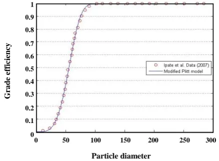
Modified Plitt’s model

To create an effective model, Plitt’s basic model which was introduced in the previous section can be employed. For this purpose, the pressure drop coefficient, C2, is optimized by minimizing the objective function

so as to find the correction factor for the pressure drop. Then, the correction factors of separation diameter, C1,

flow fraction, C3 and sharpness of the grade efficiency

slope, C5 are found by optimizing via a genetic algorithm.

To find the pressure drop coefficient, the data given by Ipate and Căsăndroiu are considered as real values and

the objective function defines as: obj



Following the determination of C2 the data proposed

for the grade efficiency with respect to solid particles diameter in the hydrocyclone (as indicated in several plots) are considered as real values and by minimizing

the objective function obj



process was done by application of the Genetic Algorithm in the platform of Matlab 10a within the variables’ interval of 0.01 <C1< 10, 1 <C2< 100,

0.01 <C3< 10, 0.01 <C4< 10, with a population of 100

and a generation value of 100.

The results of two optimization operations of the aforementioned objective function are presented in Table 3 and Fig. 18. It should be noticed that the obtained coefficients are eligible for a hydrocyclone of certain dimensions (dimensions defined by Ipate and Căsăndroiu) and that they will change for other cyclone sizes. As it is apparent from Fig. 18, the modified Plitt’s model agrees well with Ipate’s findings. Hence, this modified model has a high capability in hydrocyclone performance efficiency estimation.

CONCLUSIONS

- The results of the Numerical model taken from COMSOL Multiphysics package were compared against real measured data.

Particle diameter

0 20 40 60 80 100 120 140 160 180 200

Gra

d

e

ef

fi

ci

en

cy

1

0.9

0.8

0.7

0.6

0.5

0.4

0.3

0.2

0.1

0

Particle diameter

0 20 40 60 80 100 120 140 160 180 200

Gra

d

e

ef

fi

ci

en

cy

1

0.9

0.8

0.7

0.6

0.5

0.4

0.3

0.2

0.1

0

Particle diameter

0 50 100 150 200 250 300

Gra

d

e

ef

fi

ci

en

cy

1

0.9

0.8

0.7

0.6

0.5

0.4

0.3

0.2

0.1

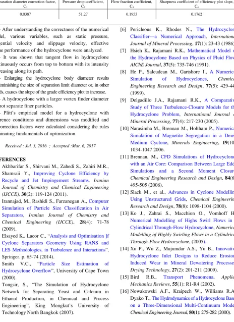
Table 3: Results of optimizing correction factors in Plitt’s model.

Separation diameter correction factor, C1

Pressure drop coefficient, C2

Flow fraction coefficient, C3

Sharpness coefficient of efficiency plot slope, C4

0.0387 51.27 0.1953 0.1762

- After understanding the correctness of the numerical model, various variables, such as static pressure, tangential velocity and slippage velocity, effective in the performance of the hydrocyclone were analyzed.

- It was shown that tangent flow in hydrocyclone continuously occurs from top to bottom with its intensity decreasing along its path.

- Enlarging the hydrocyclone body diameter results in diminishing the size of separation limit diameter or, in other words, causes the slope of the grade efficiency plot to increase.

- A hydrocyclone with a larger vortex finder diameter cannot separate finer particles.

- Plitt’s empirical model for a hydrocyclone with reference conditions and dimensions was modified and its correction factors were calculated considering the rules dominating fundamentals of optimization.

Received : Jul. 3, 2016 ; Accepted :Mar. 6, 2017

REFERENCES

[1] Akhbarifar S., Shirvani M., Zahedi S., Zahiri M.R., Shamsaii Y., Improving Cyclone Efficiency by Recycle and Jet Impingement Streams, Iranian Journal of Chemistry and Chemical Engineering (IJCCE), 30(2): 119-124 (2011).

[2] Irannajad, M., Rashidi S., Farzanegan A., Computer Simulation of Particle Size Classification in Air Separators, Iranian Journal of Chemistry and Chemical Engineering (IJCCE), 28(4): 71-78 (2009).

[3] Elsayed K., Lacor C., “Analysis and Optimisation ]f Cyclone Separators Geometry Using RANS and LES Methodologies, in Turbulence and Interactions”,

Springer. p. 65-74 (2014).

[4] Smith V.C., “Particle Size Estimation of Hydrocyclone Overflow”, University of Cape Town

(2000).

[5] Tongsir, S., “The Simulation of Hydrocyclone Network for Separating Yeast and Calcium in Ethanol Production, in Chemical and Process Engineering”, King Mongkut’s University of Technology North Bangkok (2007).

[6] Pericleous K., Rhodes N., The Hydrocyclone Classifier—a Numerical Approach, International Journal of Mineral Processing, 17(1): 23-43 (1986). [7] Hsieh K., Rajamani R.K., Mathematical Model of

the Hydrocyclone Based on Physics of Fluid Flow, AIChE Journal, 37(5): 735-746 (1991).

[8] He P., Salcudean M., Gartshore I., A Numerical Simulation of Hydrocyclones, Chemical Engineering Research and Design, 77(5): 429-441 (1999).

[9] Delgadillo J.A., Rajamani R.K., A Comparative Study of Three Turbulence-Closure Models for the Hydrocyclone Problem, International Journal of Mineral Processing, 77(4): 217-230 (2005).

[10] Narasimha M., Brennan M., Holtham P., Numerical Simulation of Magnetite Segregation in a Dense Medium Cyclone, Minerals Engineering, 19(10): 1034-1047 2006.

[11] Brennan, M., CFD Simulations of Hydrocyclones with an Air Core: Comparison Between Large Eddy Simulations and a Second Moment Closure, Chemical Engineering Research and Design, 84(6): 495-505 (2006).

[12] Slack M., et al., Advances in Cyclone Modelling Using Unstructured Grids, Chemical Engineering Research and Design, 78(8): 1098-1104 (2000). [13] Ko J., Zahrai S., Macchion O., Vomhoff H.,

Numerical Modelling of Highs Swirl Flows in a Cylindrical Through-Flow Hydrocyclone, Numerical Modelling of Highly Swirling Flows in a Cylindrical Through-Flow Hydrocyclone, (2005).

[14] Xu P., Wu Z., Mujumdar A.S., Yu B., Innovative Hydrocyclone Inlet Designs to Reduce Erosion-Induced Wear in Mineral Dewatering Processes, Drying Technology, 27(2): 201-211 (2009).

[15] Bird R.B., Transport Phenomena, Applied Mechanics Reviews, 55(1): R1-R4 (2002).

[17] Suasnabar, D.J., “Dense Medium Cyclone Performance Enhancement via Computational Modelling of the Physical Processes”, University of New South Wales (2000).

[18] Brennan, M.S., Narasimha M., Holtham P.N.,

Multiphase Modelling of Hydrocyclones–Prediction of Cut-Size, Minerals Engineering, 20(4): 395-406 (2007). [19] Hsieh K.T., Rajamani K., Phenomenological Model

of the Hydrocyclone : Model Development and Verification for Single-Phase Flow, International Journal of Mineral Processing, 22: 223-237 (1988). [20] Wang B., Yu A., Numerical Study of Particle–Fluid

Flow in Hydrocyclones with Different Body Dimensions, Minerals Engineering, 19(10): 1022-1033 (2006).

[21] Ghadirian M., Hayes R.E., Mmbaga J., Afacan A., Xu Z., On the Simulation of Hydrocyclones Using CFD, The Canadian Journal of Chemical Engineering, 91(5): 950-958 (2013).

[22] Hsu C.-Y., Wu S.-J., Wu R.-M., Particles Separation and Tracks in a Tydrocyclone, 淡江理工學刊, 14(1): 65-70 (2011).

[23] Holdich R.G., “Fundamentals of Particle Technology”, Midland Information Technology and Publishing (2002).

[24] Barth W., Brennstoff-Warme-Kraft, 8. (1956). [25] Yang W.C., “Handbook of Fluidization and

Fluid-Particle Systems”, Taylor & Francis (2003).

[26] Zenz F.A., Cyclone-Design Tips, Chemical Engineering,. 108(1): 60- (2001).

[27] Plitt L., A Mathematical Model of the Hydrocyclone Classifier, CIM Bulletin, 69(776): 114-123 (1976). [28] Hsieh K.-T., Rajamani K., Phenomenological Model of

the Hydrocyclone: Model Development and Verification for Single-Phase Flow, International Journal of Mineral Processing, 22(1): 223-237 (1988). [29] Ipate G., Căsăndroiu T., Numerical Study of Liquid-Solid Separation Process Inside the Hydrocyclones whit Double Cone Sections, Scientific Bulletin of UPB, 69: 19-28 (2007).

[30] Bhaskar K.U., Murthy Y.M., Raju M.R., Tiwari S., Srivastava J.K., Ramakrishnan N., CFD Simulation and Experimental Validation Studies on Hydrocyclone, Minerals Engineering, 20(1): 60-71 (2007).

[31] GAO S.-l., Wei D.Z., Liu W.G., MA L.Q., Lu T., Zhang R.Y., CFD Numerical Simulation of Flow Velocity Characteristics of Hydrocyclone, Transactions of Nonferrous Metals Society of China, 21(12): 2783-2789 (2011).

[32] Hoffmann P.D.A.C., Hoffmann A.C., Stein L.E., “Gas Cyclones and Swirl Tubes”, Springer (2002).

[33] Iozia, D.L., Leith D., Effect of Cyclone Dimensions on Gas Flow Pattern and Collection Efficiency, Aerosol Science and Technology, 10(3): 491-500 (1989).

[34] KOCH W.H., LICHT W., New Design Approach Boosts Cyclone Efficiency, Chemical Engineering, 84(24): 80-88 (1977).

[35] Dietz, P., Collection Efficiency of Cyclone Separators, AIChE Journal, 27(6): 888-892 (1981). [36] Hoffmann A.C., Stein L.E., Cyclone Separation

Efficiency, Gas Cyclones and Swirl Tubes: Principles, Design and Operation, 89-109 (2008). [37] Rietema, K., Het Mechanisme van de Afscheiding

van Fijnverdeelde Stoffen in Cyclonen, De Ingenieur, 71: 39- (1959).

[38] Avci A., Karagoz I., Effects of Flow and Geometrical Parameters on the Collection Efficiency in Cyclone Separators, Journal of Aerosol Science, 34(7): 937-955 (2003).