Load Balancing in Heterogeneous Cloud Environments by Using PROMETHEE Method

DOI: https://doi.org/10.30880/ijie.2018.10.08.012

Load Balancing in Heterogeneous Cloud Environments by

Using PROMETHEE Method

Samira Hourali

1

, Shahram Jamali

2

1, 2 _{Computer Engineering Department}

University of Mohaghegh Ardabili, Ardabil, Iran

1_{Electrical and Computer Engineering Department}

Non Benefit University of Shahrood Shahrood, Iran

Received 18 August 2017; accepted 29 October 2018, available online 31 December 2018

1. Introduction

Cloud computing is a new technology in academic world. In a cloud platform, resources are provided as service under a predefined Service Level Agreement (SLA) [1]. But, since the resources are shared, subscribers' requirements have big dynamic heterogeneity; the resource may be wasted if they cannot be assigned properly [2]. As other systems, dynamically balancing the load among the servers improves resource utility and the overall cloud performance in the cloud environment. Therefore, an important problem to be solved is how to dynamically and efficiently manage resources to meet the subscribers' requirements and to maximize the overall performance.

The main result of the load balancing is to speed up the execution of applications on resources whose workload varies at run time in unpredictable way [3]. Load balancing techniques are widely discussed in homogeneous as well as heterogeneous environments such as grids. There are basically two kinds of load balancing techniques, namely, static and dynamic.

Static load balancing algorithms assign the tasks to the nodes based only on the ability of the node to process new requests. The process is based solely on prior knowledge of the nodes’ properties and capabilities. These would include the node’s processing power, memory and storage capacity, and most recent known communication performance. Although they may include knowledge of the communication prior performance, static algorithms generally do not consider dynamic changes of these

attributes at run-time. In addition, these algorithms cannot adapt to load changes during run-time. Dynamic load balancing algorithms take into account the different attributes of the nodes’ capabilities and network bandwidth. Most of these algorithms rely on a combination of knowledge based on prior gathered information about the nodes in the cloud and run-time properties collected as the selected nodes process the task’s components. These algorithms assign the tasks and may dynamically reassign them to the nodes based on the attributes gathered and calculated. Such algorithms require constant monitoring of the nodes and task progress and are usually harder to implement. However, they are more accurate and could result in more efficient load balancing.

In cloud computing environments, whenever a VM is heavily loaded with multiple tasks, these tasks have to be removed and submitted to the under loaded VMs of the same data center. In this case, when we remove more than one task from a heavy loaded VM and if there is more than one VM available to process these tasks, the tasks have to be submitted to the VM such that there will be a good mix of priorities i.e., no task should wait for a long time in order to get processed. Load balancing is done at virtual machine level i.e., at intra-data center level.

We suggest that load balancing in cloud computing can be formulated as a multi-criteria decision making (MCDM) problem and then use PROMETHEE decision making algorithm to solve it. The proposed algorithm uses resources' information to compute the desired criteria (load balancing) and solve the problem. Then it directs the Abstract: Efficient Scheduling of tasks in a cloud environment improves resources utilization thereby meeting users' requirements. One of the most important objectives of a scheduling algorithm in cloud environment is a balanced load distribution over various resources for enhancing the overall performance of the cloud. Such a scheduling is complex in nature due to the dynamicity of resources and incoming application specifications. In this paper, we employ PROMETHEE decision making model to design a scheduling algorithm, called PROMETHEE Load Balancing (PLB).This paper formulates the load balancing issue as a multi-criteria decision making problem and aims to achieve well-balanced load across virtual machines for maximizing the overall throughput of the cloud. Extensive simulation results in CloudSim environment show that the proposed algorithm outperforms existing algorithms in terms of load balancing index (LBI), VM load variation, makespan, average execution time and waiting time.

virtual infrastructure manager to provide an appropriate allocation. This allocation is actually a choice between existing processing nodes based on various resources' specifications and users' requirements. The specific contributions of this paper include:

 An algorithm for scheduling and load balancing of non-preemptive independent tasks in cloud computing environments inspired by PROMETHEE decision making method.

 Correlation of the proposed PLB1 _{algorithm with}

actual PROMETHEE decision making method.  A clear flow diagram showing the PROMETHEE load balancing algorithm.

 An analysis and systematic study with mathematical evidence to show how the PROMETHEE decision making method is helpful for load balancing in the cloud computing environments.

Rest of this paper is organized as follows; Section 2 reviews the related works on existing load balancing techniques. Section 3 brings PROMETHEE decision-making method and explains it. Section 4 employs PROMETHEE to design a scheduling algorithm and presents its detailed algorithm. Section 5 presents the experimental results for performance evaluation of the algorithm in comparison with existing algorithms. Finally we conclude this paper highlighting the contributions and future enhancements in Section 6.

2.

Related Works

Load balancing is removing tasks from over loaded VMs and assigning them to under loaded VMs. It can affect the overall performance of a system executing an application. Load balancing algorithms can be classified in to dynamic and static algorithms [4]:

Static algorithms work properly only when nodes have a low variation in the load. Therefore, these algorithms are not suitable for cloud environments where load will be varying at varying times. Dynamic load balancing algorithms are advantageous over static algorithms. But to gain this advantage, we need to consider the additional cost associated with collection and maintenance of the load information.

DDFTP algorithm [5] performs load balancing by dividing the file of size n into n/2 divisions. Then, each server node starts processing the task assigned for it based on a certain pattern. When the two servers download two consecutive blocks, the task is considered as finished and other tasks can be assigned to the servers. This minimizes the node communication, thereby reducing the network overhead which further eliminates the need for run-time supervision of nodes. But attaching file divisions imposes some time complexity into the network. The proposed method finds the best server for the job taking into account all the aspects, instead of splitting the file between multiple servers.

1 _{Promethee Load Balancing}

LBMM algorithm solves the bottleneck problem, minimize execution time of each task; also avoid unnecessary replication of task on the node thereby minimizing overall completion time. In this algorithm the request manager assigning receiving task to service manager. Then service manager divide received task into subtasks. After that LBMM assigns sub-tasks to the node which requires minimum execution time [6]. In this method, several VMs are involved in the execution of a task, but in the proposed method, only one VM is used to run each task, which prevents other servers from wasting time.

In ACO2 algorithm when the request in initiated the ant start its movement [7]. Ant’s Movement is of two ways: forward movement and backward movement. This algorithm reduced the unnecessary backward movement overcome heterogeneity is excellent in fault tolerance. forward movement means the ant in continuously moving from one overloaded node to another node and check it is overloaded or under loaded, if ant find an over loaded node it will continuously moving in the forward direction and check each nodes .Backward movement: If an ant find an over loaded node the ant will use the backward movement to get to the previous node, in the algorithm if ant finds the target node then ant will commit suicide [8].

D. Babu et al [9] proposed a Honey Bee Behavior inspired Load Balancing [HBB-LB] technique which helps to achieve even load balancing across virtual machine to maximize throughput. It considers the priority of task waiting in queue for execution in virtual machines. After that work load on VM calculated decides whether the system is overloaded, under loaded or balanced. And based on this VMs are grouped. New according to load on VM the task is scheduled on VMs. Task which is removed earlier. To find the correct low loaded VM for current task, tasks which are removed earlier from over loaded VM are helpful. Forager bee is used as a Scout bee in the next steps. In this method, the waiting time may be increased slightly, which is solved in the proposed method because the Promethee technique has a high speed in finding the most suitable VM for the input task.

MapReduce algorithm adds one more load balancing level between the map job and the reduce job to decrease the overload on these jobs. The load balancing in the middle divides only the large jobs into smaller jobs and then the smaller blocks are sent to the reduce jobs based on their availability. There are three methods (part, comp and group) in this model [10]. This algorithm initiate the mapping of jobs by executes the part method. At this step the request entity is partitioned into parts using the map jobs. Then, the key of each part is saved into a hash key table and the comp method does the comparison between the parts. After that, the group method groups the parts of similar entities using the reduce jobs. Since several map jobs can read entities in parallel and process them, this will cause the reduce jobs to be overloaded. Stochastic hill climbing approach proposed to the load balancing for

maximum optimization of available resources. A local optimization approach Stochastic Hill climbing is used for allocation of incoming jobs to the servers or virtual machines (VMs) [11, 12].

A stochastic and Local Optimization algorithm is simply a loop that continuously moves in the direction of increasing value, which is uphill. It maps assignments to a set of assignments by making minor changes to the original assignment. Algorithm stops when it reaches a ”peak” where no neighbor has a higher value. This variant chooses at random from among the uphill moves and the probability of selection can vary with the steepness of the uphill move. The WRR3 _{is similar to the Round Robin in a sense}

that the manner by which requests are assigned to the nodes is still cyclical, albeit with a twist. The node with the higher specs will be apportioned a greater number of requests. This method focus in particular on algorithms based on closed queuing networks for multi-class workloads, which can be used to describe application with service level agreements differentiated across users [13].

3.

Proposed algorithm:

3.1

Cloud Environment Model

The defined space of cloud computing consists of K clusters for processing (service) .m is the number of physical servers that are shown as S= {S1,S2,…,Sm}. Let

VM(Sf)= {VM1, VM2,…,VMn}, f∈[1,m] be the set of m

virtual machines per physical server which should process z tasks represented by the set T = {T1, T2, . . ., Tz}. We

denote sending time of a task Ti by STi (0≤STj≤T).

Each processing node rj (physical server or VM) has

five characteristics which can be denoted as VMj= (rcpj,

rmj, rIOj, rcj, rnj). rcpjis processing power of each node in

other words the number of executed instructions by each node processing elements. rmj and rIOj respectively

represent the rate of utilization of memory and I/O. rcj is

the resource price and finally rnj is the amount of delay

(traffic) on the network to achieve a processing node. Each Tj task has five characteristics in this

environment which can be denoted as Tj= (cpi, mi, IOi, bi,

di). Where containing element, cpi is the rate of CPU

utilization for task Ti, mi is the rate of memory utilization

for task Ti, IOi is the rate of I/O utilization for task Ti, bi is

the fund allocated to the task Ti and di is maturity of the

task execution.

Current workload of all available VMs can be calculated based on the information received from the datacenter. Based on this, standard deviation has to be calculated to measure deviations of load on VMs.

3.2

Formulation of the problem

3.2.1

Decision matrix

As was said, load balancing in cloud computing can be formulated as a multi-criteria decision making (MCDM) problem. As shown in figure 1, the multi-criterion decision problem can be expressed in the form of

3_{Weighted Round Robin}

a decision matrix (n*5) where alternatives (a1,…, an) are

VMs which must be ordered and criteria (f1,…, f5) are

(rcpj, rmj, rIOj, rcj, rnj) which must be optimized. r_n,5is assigned value of 5th criteria for nth VM.

3.2.2

Normalized decision matrix

This step transforms various attribute dimensions into non-dimensional attributes, which allows comparisons across criteria. Normalize scores or data as follows:

2

1







r ij

N ij

n

r ij

i

₍₁₎

3.2.3

Criteria’s weights

In this paper, weight of criteria is calculated based on entropy method [14].

1. Definition of the entropy

In the 5 indicators, n evaluating objects evaluation problem, the entropy of ith indicator is defined as:

1

ln , 1, 2,...,5 

 



n 

j ij ij

j

k i

H

f

f

(2)

In which

1

1 ,

ln ij

ij n

ij j

N

f k

n N



 



, and suppose

whenf_ij 0,f_ijlnf_ij 0.

2. Definition of the weights of entropy for processing node’s criteria:

The weight of entropy of ith indicator could be defined as:

5

1 1

5

'

  





j j

j j

H

w

H

(3)

3. Definition of the final weights of task’s criteria By considering the following vector which is shown in figure 2, final weight of criteria will be calculated as follows:

' 5

' 1

i i i

i i i

p w

W

p w







(4)

In which 0

w

i1, 5

1

1







i

i

w

Fig.1 Initial Matrix P

Fig.2

Fig.2 vector J

3.2.4

Final Ranking with PROMETHEE

PROMETHEE Decision Making Method algorithm can be summarized as follows [15]:

1.To indicate for each criterion fj(a) generalized

preference function Pj(ai,ak) = fj(ai)- fj(ak) , fj(a) is the

value of jth criterion for ath alternative.

2. To define for all the alternatives ai, ak A the preference

relation P:

1

* [0,1]

:

( , ) ( ( ) ( )

n

i k j j j i j k

j

A A

a a w P f a f a

 _

  



 _{ }







(5)

The preference index p(ai,ak) is an intensity

measurement of the total preference of the decision maker for an alternative ai compared to an alternative ak and that

by taking into account all the criteria simultaneously.

3.To calculate outgoing flow which is a measure of alternative force ai∈A like:

1

1

( ) ( , )

n

i i k

i i k

a a a

n







 





(6)

4.To calculate entering flow which is a measure of the outclassed character of an alternative ai∈A, as:

1 1

( ) ( , )

n

i k i

i i k

a a a

n







 





(7)

5. Preference relation evaluation.

Basically, more the outgoing flow is large and more the entering flow is weak, better is the alternative. PROMETHEE-I method lead to a partial pre-order which is obtained by comparing the outgoing–entering flows and by carrying out the intersection between the two total pre-orders (obtained by leaving and entering flows) what makes it possible to emphasize incomparable alternatives. If a complete pre-order is necessary, PROMETHEE-II method calculates net flow like the difference between entering and outgoing flows; thus, we must avoids all incomparability between two alternatives. The alternative with the highest value of ϕ is the best option is to choose.

( )a_i ( )a_i ( )a_i



_



 _



 ₍₈₎

3.3

Standard deviation of load

Current workload of all available VMs can be calculated based on the information received from the datacenter. Based on this, standard deviation has to be calculated to measure deviations of load on VMs.

f1 f2 …. f5

Criteria Alternatives

a1

a2

. . . an

r1,1

r2,1

.

.

.

rn,1

r2,1

r2,2

.

.

.

rn,2

r1,5

r2,5

.

.

.

rn,5

…

…

…

C1 C2 C3 C4 C5

Criteria Alternative

P1 P2 P3 P4 P5

3.3.1

Capacity of a VM

i numi mipsi bwi

C



Pe



Pe



VM

(9)

Where processing element, Penumi is the number

processors in VMi, Pemipsi is million instructions per second

of all processors in VMi and VMbwi is the communication

bandwidth ability of VMi.

3.3.2

Capacity of all VMs

1

n i i

C

C







(10)

Summation of capacity of all VMs is the capacity of data center.

3.3.3

Load on a VM

Total length of tasks that are assigned to a VM is called load

.

,

( , )

(

, )

i

V M t

i

N T t

L

S V M t



(11)

Load of a VM can be calculated as the number of tasks at time t on service queue of VMi divided by the

service rate of VMi at time t. load of all VMs in a data

center is calculated as:

, 1

i t m

V M i

L

L







(12)

Processing time of a VM:

,

i V M t i

i L PT

C



(13)

Processing time of all VMs:

L PT

c



(14)

Standard deviation of load: 2

1 1

( )

m

i i

PT PT

m











(15)

3.4

Load balancing decision

After finding the workload and standard deviation, the system should decide whether to do load balancing or not. For this, there are two possible situations i.e., (1) Finding whether the system is balanced (2) Finding whether the whole system is saturated or not (The whole group is overloaded or not). If overloaded, load balancing is meaningless. Decision maker is faced with a finite n option:

VM={VMi | i=1, 2,…, n}

a.

Finding State of the VM group

If the standard deviation of the VM load (𝜎) is under or equal to the threshold condition set (Ts) [0–1] then the system is balanced [17]. Otherwise system is in an imbalance state. It may be overloaded or under loaded.

if Ts

System is balanced Exit

 

b.

Finding Overloaded Group

When the current workload of VM group exceeds the maximum capacity of the group, then the group is overloaded. Load balancing is not possible in this case

.

maximum

if L capacity

Load balancing is not possible

else

Trigger load balancing



3.4.1

PLB

In this work, each server is responsible for balancing the load of its VMs and other servers. In each server, virtual infrastructure manager is responsible for allocating resources to tasks and VMs. Therefore, the amount of server resources is always busy for that server and infrastructure manager use this resource for the calculation. The proposed method is a dynamic method that decides simultaneously to get tasks and according to dynamic information of resource.

On each server, the virtual infrastructure manager sets two tables, one is load table and another is server table, load table is the table that amount of load available for all VMs on the server and also its overall load on the server is located in. To determine the amount of the load for each resource of a processing node, Total tasks in the queue resources (CPU, Memory, I/O) is divided into the speed of each source which is obtained by following equation:

1

_ _ ( )( )

( ) (

_ ( )

Sec m

i i

job cpu length i MI load cpu

MI computing capacity







(16)

1

_ _ ( )( )

( ) (

_ ( )

Sec m

i i

job Mem length i MB

load Mem

MB

Memory bandwidth







(17)

1

_ _ ( )( )

( ) (

_ ( )

Sec m

i i

task IO length i MB

load cpu

MB IO bandwidth







(18)

tasks in the queue that source is calculated. If this value is greater than a threshold value (T) that means this resource is over loaded and otherwise it will be a light loaded resource. This concept is defined in pseudo-code:





, , /

If max CPU Mem I O T

utilization Level is High else

utilization Level is Low endif



In the server table, information of servers providing a service is existing. With addition of each physical server to cloud, this table is updated. Two main scenarios have been considered in this simulation. In the first scenario, tasks are one by one and consecutive in to a cloud (in a moment of time, there is only one task for a service and the input for other services, zero) this scenario is used to set simulation environment and the values obtained are more realistic. Servers in the cloud can provide one or more services simultaneously. If the server can provide only one service this means that all existing VMs on that server are located in a cluster and if a server simultaneously provides more than one service this means that as the number of services provided by this server, groups of VMs are existing.

With the arrival of each task to a server, infrastructure manager of that server finds the best VM for allocating the task in corresponding cluster with using the PROMETHEE decision making method. If the capacity of all VMs is full on the cluster servers using to decide the action to select the best server for the transfer of other VM's to the server for create a capacity to creation new VM.Since the proposed method uses the PROMETHEE decision making’s method for load balancing it called PLB. In this method, instead of defining an objective function to compare the resources and decision-making matrix is used.

3.4.2

Two Level Load Balancing

In this work 3PCS [18] model is considered for heterogeneous cloud computing environment, Figure 3 shows this model. The PLB load balancing algorithm is represented in two levels:

a.

VM Level:

When a task reaches to the source server, virtual infrastructure manager of source server calls for the collection of load tables from other servers within a cluster according to server table. Servers within a cluster are servers that provide the desired service by the number of VMs. Servers with receiving this call at first edit information of that part of load table that service provider VMs are there, and then send to the source server. This

edition is that eliminates all VM's that are overload from table and only VMs who have a light load (load is less than T) sends to the source server. Source server receives all the load tables that were edited as well as measuring the average maturity time for each server, make the Prometheus Matrix decision, then According to the criteria, produce weight vector (eq.4) and specifies the best VM for the allocation of input task.

b.

Physical Server Level:

After entering the task and calling the source server to collect load tables, if no VM is found, In other words, if the load tables received by the source server are empty, it Means all the VM's on the cluster are over load. At this time, the entire cluster is over load. To fix the problem, the new processing capacity (VM) should create in cluster, as part of the cluster load is transferred to it. For do this, the source server checks the amount of load of each servers in the received load tables. Servers that have empty capacity should create VM, If the server was not found to create VM, other VMs of Available servers in the cluster attempt to migrate (from other clusters) to servers of that clusters. To do this, the servers need to choose the best server to migrate the other their VM to it. Thus, the servers according to PROMETHEE algorithm and entropy weighting method (eq.3) try to choose the best server. Fig.3 shows the flowchart of two level load balancing of our algorithm.

4.

Experimental results

A cloud computing system has to handle several hurdles like network flow, load balancing on virtual machines, federation of clouds, scalability and trust management and so on. Research in cloud computing generally focus on these issues with varying importance. Cloud services have to handle the temporal variation in demand through dynamic provisioning or de provisioning from clouds. Considering all these, we can’t directly use the cloud computing system. In this section, we have analyzed the performance of our algorithm based on the results of simulation done using CloudSim. We have extended the classes of CloudSim simulator to simulate our algorithm.

Fig.3 Flow diagram of two level Load balancing (physical server and VM levels). Start (With coming task)

Creating VM on selected

server and assigning task

to it.

End Yes

No

Yes

No Collecting the load tables from other cluster by a server within the cluster, choosing the best

server by PROMETHEE method and migrating VM to it.

Creating the VM on selected server and assigning task

to it.

Collecting server tables and Remove the overloaded servers

Remains a

server?

Choosing the best server by PROMETHEE. Collecting load tables, and

removing VMs with high cost and delay

Remains a VM?

Choosing the best VM by PROMETHEE

method and assigning task

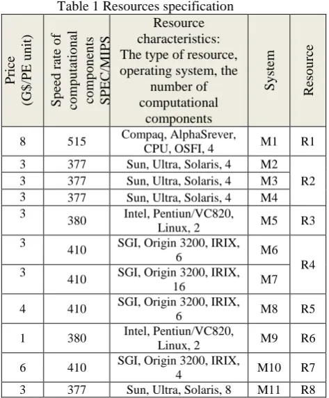
Table 1 Resources specification R eso u rce Sy stem Resource characteristics: The type of resource, operating system, the

number of computational components Sp ee d r ate o f co m p u tatio n al co m p o n en ts SP E C /MI PS Pric e (G$ /PE u n it) R1 M1 Compaq, AlphaSrever,

CPU, OSFI, 4 515

8

R2 M2 Sun, Ultra, Solaris, 4

377 3

M3 Sun, Ultra, Solaris, 4

377 3

M4 Sun, Ultra, Solaris, 4

377 3 R3 M5 Intel, Pentiun/VC820, Linux, 2 380 3 R4 M6 SGI, Origin 3200, IRIX,

6 410

3

M7 SGI, Origin 3200, IRIX,

16 410

3

R5 M8 SGI, Origin 3200, IRIX,

6 410 4 R6 M9 Intel, Pentiun/VC820, Linux, 2 380 1 R7 M10 SGI, Origin 3200, IRIX,

4 410

6

R8 M11 Sun, Ultra, Solaris, 8

377 3

When servers are purchased for a database, they are usually have the same genre and the same processing capacity. Over time, with the placement of servers, new servers with a different processing capacity may enter into the database, thus, the selection of servers has been used the normal distribution in the simulation [21].

In this simulation, fifty servers are intended that According to Table 2, resources capacity on each server is obtained by using normal distribution and the listed specifications in Table 3.

Ten services are provided by cloud, each of these services are different from each other, that means the consumption of processor resources for each of them is different, which requires considering the different levels of service mean (µ) and variance (σ2_{) in the normal}

distribution to produce VMs of services [22]. As a result, on each server, different VM groups with different resources will be placed, the mean and variance of each service is shown in Table 4. After the VMs distribution on servers, on average 514 numbers of VM is obtained.

Table 2 Resource specifications in the CloudSim tools Table 3 Servers specifications used in the simulation

Table 4 VMs Specification used in each service Table 5: Submitted tasks properties to the cloud Type of Service VM capacity CPU (MIPS) Mem. (MB/S) I/O (B/S) µ 2 σ µ 2 σ µ 2 σ 1 200 50 2 0.5 500 50 2 250 40 3 0.5 400 50 3 300 50 2 0.5 600 40 4 270 30 3 0.5 500 50 5 325 20 2 0.5 450 50 6 350 10 3 0.5 550 50 7 200 60 2 0.4 470 40 8 370 20 2 0.3 500 30 9 400 10 2 0.4 550 40 10 300 20 2 0.5 600 20

Rate of utilization of resources for any work has been obtained by the uniform distribution. For each task, level of utilization of CPU within the range (20-40) (MIPS), utilization of memory within the range (0.05-0.5) and utilization of I/O within the range (60-80) have been considered. As shown in table 6. The total number of submitted tasks to the cloud is considered equal to 100,000. The amount of funding and maturity of any task is obtained by a normal distribution function, which is mean and standard deviation is shown in Table 5.

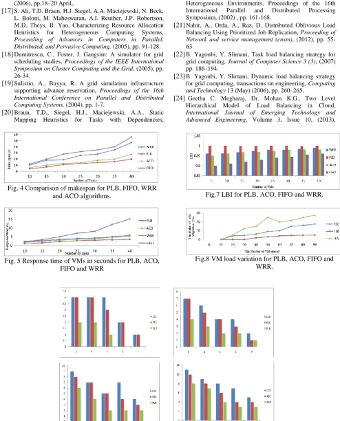
In the following illustrations, we have compared the makespan of WRR, FIFO, Ant Colony Optimization (ACO) [7, 13, 23, and 24] and our algorithm (PLB) in different low and over loaded ratios. Fig.4 shows the

comparison of makespan for PLB, FIFO and WRR, ACO. The X-axis shows the number of tasks and the Y-axis shows makespan in seconds. It is clearly evident from the graph that PLB is more efficient when compared with other 3 algorithms. Fig.5 illustrates the response time of VMs in seconds for PLB, ACO, FIFO and WRR Algorithms. The X-axis represents number of tasks and the Y-axis represents time in seconds. It is evident that PLB is more efficient compared with other three methods.

a.

Load Balancing Index (LBI):

To evaluate the performance metric of our load balancing algorithm (PLB), In order to decide whether the

network needs to be balanced, it uses the load balancing index (LBI), which is calculated by the following equation: 2 1 2 1 ( ) n i i n i i U LBI N U   





(19) Where N is the number of VMs and Ui is utilization

of VMi. The purpose of PLB algorithm is to distribute the query load L fairly among the virtual machines. Figure 7 shows the relation of the VM numbers and the LBI. The value of the fairness index ranges between 0 and 1. A totally fair load distribution has a fairness index of 1 and the fairness index of a totally unfair load distribution is 0.Given the above definition, one can verify that if the VMs have the same utilization, workload is distributed to nodes proportional to their capacities; this distribution of workload is totally fair. In FIFO and ACO and WRR algorithms, when the VM number increases, the total traffic load will increase. However, the LBI is not growing worse significantly. That is, our proposed PLB schemes cloud maintain almost ideal load-balanced state and perform better load balancing than FIFO and ACO and WRR do. In addition, the LBIs of ACO and WRR will increase a little when the node number increases. Figure 6

and 7 shows the LBI for WRR, ACO, FIFO and our algorithm.

b.

VM Load Variation:

To better test the stability of the algorithm, we define VM load variation rate as α which indicates the variation range of VM load. Suppose the initial VM load deployed is LVMi,t0 and the current VM load is LVMi,t, From Eq. (11)

we can imply Eq. (20), where ∝ is VM load variation:

0 0 , , , i i i

V M t V M t

V M t

L

L

L







₍₂₀₎

The experiment mainly analyzes the load balancing effect of the algorithm and the migration cost to realize the system load balancing after scheduling by the algorithm, and makes relevant comparisons between this algorithm and the current VM balancing scheduling methods including the Rotation scheduling algorithm and Least Connection Scheduling.

On some special occasions, there is a big increase of the load of some nodes in the system due to frequent access thus leads to the load imbalance of the whole system. Under this situation, usually the system cannot realize the system load balancing through only one-time scheduling so it must do it through VM migration. However, the cost of VM migration cannot be neglected. Thus where the VM should be migrated and how to

migrate the least number of VM are also the problems that need consideration during VM scheduling. The algorithm of this paper takes historical factors into consideration. It computes the situation of the whole system after scheduling in advance through PROMETHEE algorithm and then chooses the scheduling solution with the lowest cost. Figure 8 shows the average VM migration ratio while the VM load variation rate α is changing. It can be seen that the method of this paper shows conspicuous advantage. The experiment shows that the method of this paper can greatly bring down the migration cost. Figure 9(a)–(d) shows the comparisons of task migration vs. number of virtual machines when numbers of tasks are varied from 10 to 80. Results illustrate that PLB is more efficient with lesser number of task migrations when compared with LCS and RSC [25] techniques.

5.

Conclusion

This paper presented a scheduling strategy on VM load balancing based on PROMETHEE decision making method for cloud computing environments. In this algorithm, this allocation is a choice between existing processing nodes that is proposed for the task, which uses various specifications of quality and quantity of resources based on user needs can be done. The weight of criteria is calculated based on entropy method which is effective for all the positive and negative aspect. The best appropriate VM or physical server selects based on the value of the criteria’s weights. We have compared our proposed algorithm with other existing techniques. Results show our algorithm can better realize load balancing and proper resource utilization and stands good without increasing additional overheads for balancing non-preemptive independent tasks. This load balancing technique provides minimum node idle time, handle heterogeneous resources and works well for heterogeneous cloud computing systems, the 3PCS model is considered for this environment. In future work, we plan to use learning algorithms such as the neural network, instead of using the entropy method to abtain criteria’s weight. Certainly, in this section, the training of the neural network will be important. In addition to the criteria in this project, we can include criteria such as bandwidth, etc. in the decision matrix. This will make the decisions made more accurate.

References

[1] Michael Armbrust, Armando Fox, Rean Griffith, Anthony D. Joseph, Randy Katz, Andy Konwinski, Gunho Lee, David Patterson, Ariel Rabkin, Ion Stoica, and Matei Zaharia, Above the clouds: A berkeley view of cloud computing, UC Berkeley Technical Report UCB/EECS-2009-28, February (2009).

[2] Borja Sotomayor, Kate Keahey, and Ian Foster, Overhead matters: A model for virtual resource management, In VTDC '06: Proceedings of the 1st

International Workshop on Virtualization

Technology in Distributed Computing, Washington, DC, USA (2006), page 5.

[3] D.L. Eager, E.D. Lazowska, J. Zahorjan, Adaptive load sharing in homogeneous distributed systems,

The IEEE Transactions on Software Engineering 12, Volume (5), (1986), pp.662–675.

[4] A. Revar, M. Andhariya, D. Sutariya, M. Bhavsar, Load balancing in grid environment using machine learning-innovative approach, International Journal of Computer Applications, Volume 8, (10 (Oct)) (2010), pp. 975–8887.

[5] J. Al-Jaroodi, and N. Mohamed, DDFTP: Dual-Direction FTP, 11th IEEE/ACM International Symposium on Cluster, Cloud and Grid Computing (CCGrid), IEEE (2011), pp. 504-503.

[6] S. C. Wang, K. Q. Yan, W. P. Liao and S. S. Wang, Towards a load balancing in a three-level cloud computing network, 3rd International Conference on. Computer Science and Information Technology (ICCSIT), IEEE, Volume 1, July (2010), pp. 108-113.

[7] Ren Gao, and Juebo Wu, Dynamic Load Balancing Strategy for Cloud Computing with Ant Colony Optimization, Future Internet , Volume 7, (2015), pp. 465-483.

[8] Z. Zhang, X. Zhang, A Load Balancing Mechanism Based on Ant Colony and Complex Network Theory in Open Cloud Computing Federation, Proceedings of 2nd International Conference on Industrial Mechatronics and Automation (ICIMA), Wuhan, China, (2010), pp. 240-243. L.D. DhineshBabu, P. Venkata Krishna, Honey Bee behavior inspired load balancing of tasks in cloud computing environments, Applied Soft Computing 13, (2013), pp. 2292–2303.

[9] T. Gunarathne, T-L. Wu, J. Qiu and G. Fox, MapReduce in the Clouds for Science, in proc. 2nd International Conference on Cloud Computing Technology and Science (Cloud Com), IEEE (2010), pp. 565-572.

[10] V. P. Shilpa, T. S. Shilpa, Survey on Load Balancing in Cloud Computing, International Conference on Computing,

Communication and Energy Systems (ICCCES-2014),

(2014).

[11]B. M. K. Dasguptaa, P. Duttab, Load Balancing in Cloud Computing using Stochastic Hill Climbing-A Soft Computing Approach, Procedia Technology 4 ( 2012 )

2212-0173 © 2012 Published by Elsevier Ltd.

doi:10.1016/j.protcy.2012.05.128 C3IT-(2012), pp. 783 – 789.

[12]Wang W, Casale G, Evaluating weighted round robin load balancing for cloud web services, Symbolic and Numeric Algorithms for Scientific Computing (SYNASC), 2014 16th International Symposium on, (2014).

[13]Xiaona Ren, Rongheng Lin,Hua Zou, a dynamic load balancing strategy for cloud computing platform based on exponential smoothing forecast, Proceedings of IEEE CCIS2011, (2011), pp.220-224.

[14]Zhi-hong.Z, Y. Yi, S. Jing-nan, Entropy method for determination of weight of evaluating in fuzzy synthetic evaluation for water quality assessment, Journal fo environ mental science, Volume 18, No. 5, (2006), pp.1020-1023. [15]J. P. Brans, PH.Vincke, a Preference Ranking Organization

method (The PROMETHEE Methos for Multiple Criteria Decision-Making), Management Science, volume 31, (1985), pp. 647-656.

[16]R.F. de Mello, L.J. Senger, L.T. Yang, A routing load balancing policy for grid computing environments, in: 20th

Networking and Applications, AINA(2006) 6, volume 1, (2006), pp.18–20 April,.

[17]S. Ali, T.D. Braun, H.J. Siegel, A.A. Maciejewski, N. Beck, L. Boloni, M. Maheswaran, A.I. Reuther, J.P. Robertson, M.D. Theys, B. Yao, Characterizing Resource Allocation Heuristics for Heterogeneous Computing Systems, Proceeding of Advances in Computers in Parallel, Distributed, and Pervasive Computing, (2005), pp. 91-128. [18]Dumitrescu, C., Foster, I. Gangsim: A simulator for grid

scheduling studies, Proceedings of the IEEE International Symposium on Cluster Computing and the Grid, (2005), pp. 26-34.

[19]Sulistio, A., Buyya, R. A grid simulation infrastructure supporting advance reservation, Proceedings of the 16th International Conference on Parallel and Distributed Computing Systems, (2004), pp. 1-7.

[20]Braun, T.D., Siegel, H.J., Maciejewski, A.A.. Static Mapping Heuristics for Tasks with Dependencies,

Priorities, Deadlines, and Multiple Versions in Heterogeneous Environments, Proceedings of the 16th International Parallel and Distributed Processing Symposium, (2002) , pp. 161-168.

[21]Nahir, A., Orda, A., Raz, D. Distributed Oblivious Load Balancing Using Prioritized Job Replication, Proceeding of Network and service management (cnsm), (2012), pp. 55-63.

[22]B. Yagoubi, Y. Slimani, Task load balancing strategy for grid computing, Journal of Computer Science 3 (3), (2007) pp. 186–194.

[23]B. Yagoubi, Y. Slimani, Dynamic load balancing strategy for grid computing, transactions on engineering, Computing and Technology 13 (May) (2006), pp. 260–265.

[24] Geetha C. Megharaj, Dr. Mohan K.G., Two Level Hierarchical Model of Load Balancing in Cloud, International Journal of Emerging Technology and Advanced Engineering, Volume 3, Issue 10, (2013).

Fig.9 (a) Comparison of number of task migrations vs. number of virtual machines for a set of 10 tasks. (b) Comparison of number of task migrations vs. number of virtual machines for a set of 20 tasks. (c) Comparison of number of task migrations vs. number of virtual machines for a set of 40 tasks. (d) Comparison of number of task migrations vs. number of virtual machines for a set of 80 tasks.

Fig. 4 Comparison of makespan for PLB, FIFO, WRR and ACO algorithms.

Fig. 5 Response time of VMs in seconds for PLB, ACO, FIFO and WRR

Fig.7 LBI for PLB, ACO, FIFO and WRR.