Community Microgrid Scheduling Considering
Network Operational Constraints and Building
Thermal Dynamics
Guodong Liu1*, Thomas B. Ollis1, Bailu Xiao1, Xiaohu Zhang2and Kevin Tomsovic2,
1 Power & Energy Systems Group, Oak Ridge National Laboratory, Oak Ridge, TN 37831, USA; [email protected]; [email protected]; [email protected]
2 Department of Electrical Engineering and Computer Science, The University of Tennessee, Knoxville, TN 37996, USA; [email protected]; [email protected]
* Correspondence: [email protected]; Tel.: +1-865-241-9732
Abstract: This paper proposes a Mixed Integer Conic Programming (MICP) model for community microgrids considering the network operational constraints and building thermal dynamics. The proposed multi-objective optimization model optimizes not only the operating cost, including fuel cost, purchasing cost, battery degradation cost, voluntary load shedding cost and the cost associated with customer discomfort due to room temperature deviation from the set point, but also several performance indices, including voltage deviation, network power loss and power factor at the Point of Common Coupling (PCC). In particular, the detailed thermal dynamic model of buildings is integrated into the distribution optimal power flow (D-OPF) model for the optimal operation. The heating, ventilation and air-conditioning (HVAC) systems can be scheduled intelligently to reduce the electricity cost while maintaining the indoor temperature in the comfort range set by customers. Numerical simulation results show the effectiveness of the proposed model and significant savings in electricity cost with network operational constraints satisfied.
Keywords: community microgrids; distribution optimal power flow; multiobjective optimization; thermal dynamic model; HVAC
1. Introduction
A microgrid can be defined as a low voltage distribution network comprising various distributed generation (DG), storage devices, and responsive loads that can be operated in both grid-connected and islanded modes [1]. It is connected to the main distribution network at the Point of Common Coupling (PCC), importing or exporting power to the distribution network as well as providing ancillary services, such as, voltage support, to the main distribution grid [2,3]. A microgrid can also improve local reliability, reduce emissions and contribute to lower cost of energy supply by taking advantage of the DG, storage devices and responsive loads [4]. Due to such benefits, the microgrid has attracted growing attention from both academia and industry [5].
The scheduling of microgrids in both grid-connected and islanded modes is usually performed by a microgrid controller. It determines the optimal dispatch of DG and the power exchanged between microgrid and distribution utility through PCC by solving a economic dispatch or unit commitment problem. The total operating cost is minimized subject to various technical, environmental, reliability and operating constraints. Considerable efforts have been devoted to optimal scheduling and management of microgrids [6]. Scheduling methods for a microgrid in islanded modes are proposed in [7]-[10]. In addition, numerous research and published works are devoted to the scheduling of microgrid in grid-connected mode [11]-[15]. In particular, deterministic models are used in [11] and [12], while stochastic programming models have been developed in [13]-[14]. A hybrid stochastic/robust programming model for microgrid scheduling is proposed in [15]. However, in most of existing literature, network configuration, reactive power flow and power factor constraints have been mostly ignored in the optimization model. Under this
assumption, the voltage and power factor limits as well as line thermal limits may not be satisfied by the solution. For this reason, economic and secure operation of a microgrid requires solving a distribution optimal power flow (D-OPF) considering the distribution network, voltage and power factor limits, and so on. Various approaches have been proposed for solving the D-OPF problem. Generally, these approaches can be classified into three categories. In the first category, the nonlinear optimization problem is directly solved using nonlinear programming methods such as gradient search or interior point methods [16]-[18]. It should be noted that the solution time and convergence characteristic of nonlinear programming in solving the D-OPF problem may not satisfy the stringent time constraints required by real-time controls. More commonly, as in the second category, the nonlinear optimization problem is addressed by iteratively solving the linearized problem [19]-[23]. These linear programming based methods are generally more efficient in term of solution time. Nevertheless, the linearized problem is formulated based on the calculated sensitivity coefficients, which cannot represent the nonlinear system correctly when the solution is close to the optimum. As a result, the solution may oscillate around the optimum and fail to converge. In the third category, the non-linear/non-convex items in the D-OPF problems are directly approximated or relaxed into linear/convex form. Thus, the D-OPF is formulated as linear programming [24,25]; or semidefinite programming (SDP) [26]; or second-order cone programming (SOCP) using either polar coordinates [27] or the DistFlow model [28,29] by several convex relaxations. The relaxed convex D-OPF preserves the accuracy of the power flow model while improving the solution efficiency, and thus, it has become more and more popular in recent years.
In the existing literature, HVAC consumption is mostly considered as a responsive load, which could be postponed, or as a simple non-controllable load. The thermal dynamic characteristics of buildings as well as the customer comfort preference are seldom taken into account. In fact, the slow thermal dynamic characteristic of buildings make HVAC systems perfect candidates for demand side management due to building thermal inertia. Given indoor temperature settings (desirable temperature and allowable temperature deviation) from customers, the HVAC system can precool (or preheat) the building by turning on during low price hours and turning off during high/peak price hours while still maintaining the indoor temperature in allowable range. By integrating the thermal dynamic model of buildings into the microgrid scheduling process and allowing the microgrid controller surrogate control of the HVAC systems, significant savings in electricity cost can be achieved while preserving comfort. Recently, optimal control schemes for HVAC considering thermal dynamic model of buildings has been proposed in [30]-[31]. Nevertheless, the HVAC system was modeled as a continuous controllable load, while in practical cases, most HVAC systems can only be switched on and off. In addition, the network configuration, voltage and power factor limits are neglected.
In this paper, we propose a new mixed integer conic programming (MICP) model for community microgrids considering the network operational constraints and building thermal dynamics. The proposed optimization framework optimizes not only the total operating cost, but also the performance indices, including voltage deviation, network power loss and power factor. Detailed thermal dynamic characteristics of buildings and HVAC system models are integrated into the proposed community microgrid scheduling model. The main contributions of this paper are as follows:
• proposing a multiobjective optimization model to optimize both the operating cost and performance indices of a microgrid. The weighting coefficients of each objective are determined using the analytical hierarchy process (AHP) [32].
• integrating the building thermal dynamics and HVAC systems controller into microgrid scheduling model and reducing operating cost of microgrids; and
• validating the proposed model with numerical simulation results.
scheduling model considering network operational constraints and building thermal dynamics is proposed in Section III. In Section IV, case studies and sensitivity analysis on a community microgrid are presented. Finally, conclusions are given in Section V.
2. System Modeling
2.1. Community Microgrid Model
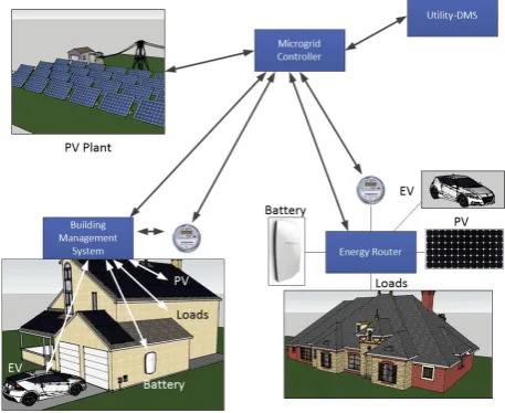
In this paper, we consider a community microgrid that consists of various distributed generation (PV panels, microturbines, fuel cells, diesel generations, etc.), energy storage (e.g., batteries) and a number of houses. For each house, there are HVAC loads and non-HVAC loads. In addition, rooftop PV panels, small batteries and EVs may also be present. A building energy management system (BEMS) is equipped for each house to communicate with the microgrid controller. Generally, the objective of the microgrid controller is to minimize the total cost of operating the community microgrid by coordinating the DG and battery operation, customers’ consumption and energy purchasing/selling at the PCC while preserving customers’ comfort and satisfying operational constraints. In particular, we assume the microgrid controller collects customer indoor temperature settings (desirable temperature and allowable temperature deviation) and other required information from each BEMS. Based on the customer requirements, electricity demand, renewable generation and price information at the PCC, the microgrid controller decides the real and reactive power output of controllable DG, charging/discharging power of batteries, purchasing/selling power at PCC and power consumption of HVAC systems as well as other controllable loads over a scheduling period (e.g., 24 hours). An example of the community microgrid under consideration is shown in Figure1.
Figure 1.Example community microgrid
2.2. HVAC System Model
Different from the autonomous temperature control above, we assume the desirable temperature and allowable temperature range set by customers are forwarded to the community microgrid controller by the BEMS and the microgrid controller takes surrogate control of HVAC systems. Since indoor temperature changes quite slowly due to thermal inertia, a house can be considered as a thermal storage facility. This gives the microgrid controller certain flexibility to schedule the consumption of HVAC system. Specially, a microgrid controller can switch on HVAC systems during low price or high renewable generation intervals to precool (or preheat) the house and switch off in opposite cases while still maintaining the indoor temperature in allowable range. As a result, it is expected that significant savings in electricity cost can be achieved compared to autonomous temperature control.
2.3. Building Thermal Dynamic Model
Thermal energy is transferred from a higher temperature space toward a lower temperature space due to conduction, convection, and radiation. Based on heat transfer mechanisms, we construct a third order linear model for the thermal dynamics of a house considering the impact of ambient temperature, solar irradiance and HVAC systems [33] as:
CMh dT M h dt =
1
RMh
ThIn−ThM+AhpshΦsh (1)
ChEdT E h dt =
1
RE h
ThIn−ThE+ 1
REA h
TA−ThE (2)
ChIndT In h
dt =
1
RA h
TA−ThIn+ 1
RMh
ThM−ThIn
+ 1
RE h
ThE−ThIn+Ah(1−psh)Φsh+
uHht−uChtηhPhH (3)
The equivalent thermal parameters RAh,RMh, REh,REAh ,ChIn,CMh,ChE, and psh are assumed to be constant for a househ, which can be estimated by using various methods based on measured data [34,35]. Thus, the above thermal dynamics of househcan be rewritten in the linear state-space model in continuous time as:
dTh
dt = AhTh+BhUh (4)
whereTh = ThIn,ThM,ThE
is the state vector. Uh = TA,Φ, uHh −uCh
ηhPhH
is the input vector. The coefficients of matricesAhandBhof a househcan be calculated based on the effective window
area, the fraction of solar irradiation entering the inner walls and floor, the thermal capacitance and resistance parameters of the house. The state-space model in continuous time (4) can be further transformed into equivalent discrete time model (5) by using Euler discretization (i. e., zero-order hold) with a sampling time [33,36], which is the time resolution of the optimization horizon
Th,t+1= AdhTh,t+BdhUh,t ∀h,∀t (5)
Where Adh and Bdh are constant, which can be calculated based on Ah, Bh and the sampling time.
This discrete time thermal dynamic model will be used in the following problem formulation. More details on this building thermal dynamic model can be found in [33]. The constraints on house indoor temperature are:
3. Problem Formulation
3.1. Objective
In the context of microgrids, dispatchable and undispatchable generation as well as batteries are integrated into the distribution network. The microgrid is connected to the external distribution system via the PCC characterized by a forecast day-ahead hourly cost of energy exchange known for a time window of 24 hours. Depending on unit type, dispatchable units are subject to various constraints, such as, capacity limits, minimum power output limits, ramping rates, minimum on/off time, and so on. In contrast, renewable generation, such as PV panels, are taken as non-dispatchable units, which depend on the meteorological conditions of ambient temperature and solar irradiance.
Each house or building is associated with a HVAC load and a non-HVAC load. Under this
assumption, the operation objective of a microgrid aims at minimizing a virtual cost associated with the system operating cost and performance as in (7). Specifically, the first and second line is the fuel cost of DGs (including DG start-up cost); the third line is the discomfort cost of customers due to the deviations between actual temperature and customer desired temperature and cost of load shedding; the fourth line is the energy purchasing/selling cost/benefit from distribution grid and cost of battery degradation; the fifth and sixth lines are total voltage deviation; and the seventh line is the total network loss and the total absolute value of reactive power exchange, which indicates the power factor at the PCC. These objectives are combined into a single objective function by a weighted summation.
min WC
(N
T
∑
t=1 NG
∑
i=1
" N
I
∑
m=1
λit(m)pit(m) +κiuit
#
+
NT
∑
t=1 NG
∑
i=1
SUit(uit,ui,t−1)
+
NT
∑
t=1 NH
∑
h=1
ωht T In ht−ThtD
+V
LS ht PhtLS
+
NT
∑
t=1
λPCCt PtPCC+
NT
∑
t=1 NB
∑
b=1 Cbt
PbtC+PbtD
)
+WV
"N
T
∑
t=1 NN
∑
n=1
Vnt2 −(Vthrmax)2: (Vnt >Vthrmax)
+
NT
∑
t=1 NN
∑
n=1
Vthrmin2−Vnt2 : (Vnt <Vthrmin)
#
+WL
"N
T
∑
t=1 NF
∑
j=1 rflf t
#
+WQ
NT
∑
t=1
Q PCC t ! (7)
The weighting coefficients WC, WV, WL and WQ can be determined by using the analytical
3.2. Constraints
The objective function must be minimized subject to a number of constraints. For simplicity, these constraints are grouped into DG constraints, battery constraints, load constraints, network constraints and constraints at PCC.
3.2.1. DG Constraints
The constraints associated with DGs include the following:
Pit = NI
∑
m=1
pit(m) +uitPimin ∀i,∀t (8)
0≤ pit(m)≤pmaxit (m) ∀i,∀t,∀m (9)
Pit≤Pimaxuit ∀i,∀t (10)
−tan(θi)Pit≤Qit≤tan(θi)Pit ∀i,∀t (11)
(Pit)2+ (Qit)2≤S2i ∀i,∀t (12)
Constraints (8) and (9) approximate the fuel cost of DGs by blocks. Constraint (10) enforces the output of DG to be zero if it is not committed. The power factor and capacity limit is ensured by (11) and (12).
3.2.2. Battery Constraints
The constraints associated with batteries include the following:
0≤PbtC ≤PbC,maxuCbt ∀b,∀t (13)
0≤PbtD≤PbD,maxuDbt ∀b,∀t (14)
uCbt+uDbt ≤1 ∀b,∀t (15)
SOCbt =SOCb,t−1+PbtCηCb4t−PbtD
1
ηbD
4t ∀b,∀t (16)
SOCbtmin≤SOCbt≤SOCmaxbt ∀b,∀t (17)
−tan(θbC)PbtC≤Qbt≤tan(θCb)PbtC :
PbtC>0∀b,∀t (18)
−tan(θbD)PbtD≤Qbt ≤tan(θDb)PbtD:
PbtD>0∀b,∀t (19)
Pbt =PbtD−PbtC∀b,∀t (20)
Constraint (13) and (14) are the maximum charging/discharging power of a battery. These two states are mutually exclusive, which is ensured by (15). The state of charge (SOC) limits are enforced by (16) and (17). In (16), the battery SOC at the end of current time interval equals to the SOC at the end of last time interval plus the energy charged minus the energy discharged during current interval. The charging and discharging of battery is subject to loss, which is represented by parameterηCb and ηDb. The power factor limits of a battery in both charging and discharging states are represented by (18) and (19). The capacity limit is ensured by (20) and (21). The logical constraints (18) - (19) will be simplified into mixed integer linear (MIL) format in subsection3.3.
3.2.3. Load Constraints
For each house, the load is divided into HVAC load and non-HVAC load as in equation (22) and (23). The constraints associated with HVAC systems include equation (5) and (6). Since the heating and cooling states of a HVAC system are mutually exclusive, this is ensured by (24). The amount of load curtailment in househat timetis limited by constraint (25) and (26).
Pht=
uHht+uChtPhH+PhtO ∀h,∀t (22)
Qht=tan
ϕHh uHht+uCht
PhH+QOht ∀h,∀t (23)
uHht+uCht≤1 ∀h,∀t (24)
0≤PhtLS≤PhtLS,max ∀h,∀t (25)
QLSht =tanϕOh
PhtLS ∀h,∀t (26)
3.2.4. Network Constraints
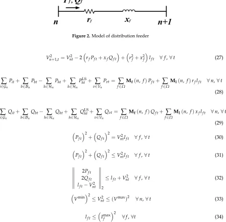
The model of a distribution feeder with busnas sending end and busn+1 as receiving end is shown in Figure2. Considering the power flow direction as depicted in Figure2. Equation (27) -(30) represents the DistFlow equations, which have been verified in [26,29]. The nodal voltage drop along a feeder is represented by (27). The real and reactive power balances across the network are enforced by (28) and (29), whereMf and Mlare the incidence matrix for the sending end line flow and line losses. Mf(n, f)is 1 if bus nis the sending end of line f, and -1 if busn is the receiving end of line f and zero if neither terminal of line f is connected to bus n. Ml(n, f)is 1 if bus nis the receiving end of line f and zero for all other elements. It should be noted thatPtPCCand QPCCt
Figure 2.Model of distribution feeder
Vn2+1,t=Vnt2 −2
rfPf t+xfQf t
+r2f +x2flf t ∀f,∀t (27)
∑
i∈Gn
Pit+
∑
b∈BnPbt−
∑
h∈HnPht+
∑
h∈HnPhtLS+
∑
v∈Vn
Pvt=
∑
f∈ΩMf(n, f)Pf t+
∑
f∈ΩMl(n, f)rflf t ∀n,∀t
(28)
∑
i∈Gn
Qit+
∑
b∈BnQbt−
∑
h∈HnQht+
∑
h∈HnQLSht +
∑
v∈Vn
Qvt=
∑
f∈ΩMf(n, f)Qf t+
∑
f∈ΩMl(n, f)xflf t ∀n,∀t
(29)
Pf t
2
+Qf t
2
=Vnt2lf t ∀f,∀t (30)
Pf t
2
+Qf t
2
≤Vnt2lf t ∀f,∀t (31)
2Pf t
2Qf t lf t−Vnt2
2
≤lf t+Vnt2 ∀f,∀t (32)
Vmin2≤Vnt2 ≤(Vmax)2 ∀n,∀t (33)
lf t≤
Imaxf 2 ∀f,∀t (34)
3.2.5. Constraints at PCC
At the PCC, the exchanged power at PCC is subject to a maximum value due to line capacity or reliability requirements as in (35). The power factor limit at PCC is ensured by (36). In addition, the PCC voltage is normally determined by the utility network operating condition, which is specified in (37) .
−PPCC,max ≤PtPCC≤PPCC,max ∀t (35)
−tan(θPCC,max) P PCC t ≤Q PCC
t ≤tan(θPCC,max)
P PCC t (36)
VtPCC=VFix (37)
3.3. Simplification and Linearization
DGs (line 2) can be recast into mixed-integer linear form as in [39]. The logic expression of voltage deviation (line 5 and 6) can be reformulated into linear format as in (38) - (40) by introducing auxiliary variableXVnt, which represents the voltage deviation. Similarly, the expression of customer discomfort cost (line 3) can be reformulated into linear format as in (41) - (43) by introducing an auxiliary variableXht, which represents the absolute value of temperature deviation. The same technique can
linearize other absolution functions in equation (7) and (36) into linear format. Thus, the proposed optimization becomes a MILP, which can be solved efficiently by commercial solvers.
XntV ≥Vnt2 −(Vthrmax)2 ∀n,∀t (38)
XVnt≥
Vthrmin2−Vnt2 ∀n,∀t (39)
XVnt ≥0 ∀n,∀t (40)
Xht≥ThtIn−ThtD ∀h,∀t (41)
Xht≥ThtD−ThtIn ∀h,∀t (42)
Xht≥0 ∀h,∀t (43)
The logical terms in battery constraints (18) and (19) can be reformulated into MIL form, as (44) and (45) by the reuse of binary charging/discharging indicators
−SbuDbt−tan(θbC)PbtC≤Qbt ≤tan(θCb)PbtC+SbuDbt∀b,∀t (44)
−SbuCbt−tan(θbD)PbtD≤Qbt ≤tan(θDb)PbtD+SbuCbt∀b,∀t (45)
Finally, the objective function has been reformulated into MIL form and all constraints are either MIL or second order cones (SOC) . Thus, the proposed D-OPF problem is represented as a MICP, which can be solved by commercial solvers efficiently.
4. Case Studies
The proposed community microgrid scheduling model is demonstrated on a modified ORNL Distributed Energy Control and Communication (DECC) lab microgrid test system as shown in Figure3. The modified system includes various DERs, including PV panel, fuel cell, microturbine, diesel generator and battery. The parameters for the dispatchable generators, PV, wind turbine and battery can be found in [15]. The three dispatchable generators are duplicated to make sure the microgrid can be operated in islanded mode without load shedding. The solar irradiance and temperature data is from [40]. The measured 1-minute data of Oak Ridge, Tennessee area on August 1st, 2015 is used for the simulation. This is a typical summer day in southern states of the US. The cost of load shedding is set as $2.0/kWh and the amount of curtailed load should be less than 10% of the corresponding non-HVAC load in each house. Twenty houses are considered, each has a 5 kW HVAC system, which has a coefficient of performance (COP)ηh=3. The desired indoor temperature
a battery. On the demand side, it considers multiple houses with different parameters. Thus, the modified DECC lab microgrid system covers a wide variety of both existing and future community microgrids components.
ƵƐϭ
ƵƐϮ
ƵƐϯ
ƵƐϰ
ƵƐϱ
Wsϭ
W
'ϭͲϯ
Ε
^ϭ
Ε
'ϰͲϲ
,ϭͲϱ
,ϲͲϭϬ
,ϭϭͲϭϱ
,ϭϲͲϮϬ
ϱϬŬt ϱϬŬtͬϭϬϬŬtŚ
ϲϬͬϯϬͬϯϬŬt ϲϬͬϯϬͬϯϬŬt
Ϭ͘ϬϭϭнũϬ͘Ϭϭϴё Ϭ͘ϭϯϰнũϬ͘Ϭϲϳё Ϭ͘ϬϭϭнũϬ͘Ϭϭϴё Ϭ͘ϭϯϰнũϬ͘Ϭϲϳё
Figure 3.Community microgrid test system
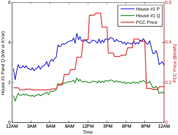
The analysis is conducted for a 24-hour scheduling horizon and the time interval is set to be 15 minutes. The PV model is the same as in [18]. The forecast non-HVAC demand in house #1 and the day-ahead market prices at the PCC are shown in Figure4. The non-HVAC load curves of other houses are assumed the same. The power factor of HVAC is assumed 0.9 and the power factor at PCC is required to be no less than 0.9. All numerical simulations are coded in MATLAB and solved using the MICP solver CPLEX 12.6. With a pre-specified duality gap of 0.5%, the running time is about 1 minute on a 2.66 GHz Windows-based PC with 4 G bytes of RAM.
12AM0 3AM 6AM 9AM 12PM 3PM 6PM 9PM 12AM
2 4 6
Time
H
o
u
s
e
#
1
P
a
n
d
Q
(
k
W
o
r
K
V
a
r)
12AM 3AM 6AM 9AM 12PM 3PM 6PM 9PM 12AM0
0.2 0.4 0.6
P
C
C
P
ri
c
e
(
$
/k
W
h
)
House #1 P
House #1 Q PCC Price
4.1. Effect of Weighting Factors
As mentioned above, the weighting coefficients of each term in the objective function are determined by using the AHP. For simplicity, fuel cost, purchasing cost, battery degradation cost, load shedding cost and customers’ discomfort cost are aggregated together as total cost with weighting coefficientWC. First of all, a pairwise comparison of relative importance or priority between each two
objectives is done. A pairwise comparison matrix can be established as in Table1. For each position in the matrix, the importance of the objective at the left is compared with that of the objective at the top and the ratio is entered. Then, the AHP retrieves the weighting coefficients of all objectives by solving a trivial eigenvalue problem. If the pairwise comparison matrix is consistent, it is rank one and thus all its eigenvalues but one are equal to zero. This largest eigenvalue, i.e., principal eigenvalue is unique and equals to the dimension of the matrix. The corresponding eigenvector, i.e., principal eigenvector is positive and unique. The weighting coefficients of objectives can be obtained by normalizing this principal eigenvector. Since each element in the pairwise comparison matrix is directly estimated by comparing the priority of two corresponding objectives, the pairwise comparison matrix is very unlikely to be consistent, especially when the number of objective is large. According to [32], a consistency of about 10% is considered acceptable. In the inconsistent case, the principal eigenvalue is still unique and near the dimension of the matrix. The weighting coefficients of objectives can be obtained in the same way.
Based on the pairwise comparison matrix in Table1, the weighting coefficients of each term are calculated as:WC=0.2084,WQ=0.1171,WV=0.6116, andWL=0.0629. It should be noted that the system
operator can change the pairwise comparison matrix according to their system configuration and preference, and then the calculated weighting coefficients will be changed, accordingly.
Table 1.Pairwise comparisons of the objective terms
Total Cost
Total Reactive
Power
Voltage Deviation
Network Loss
Total Cost 1 2 1/3 3
Total Reactive Power 1/2 1 1/5 2
Voltage Deviation 3 5 1 10
Network Loss 1/3 1/2 1/10 1
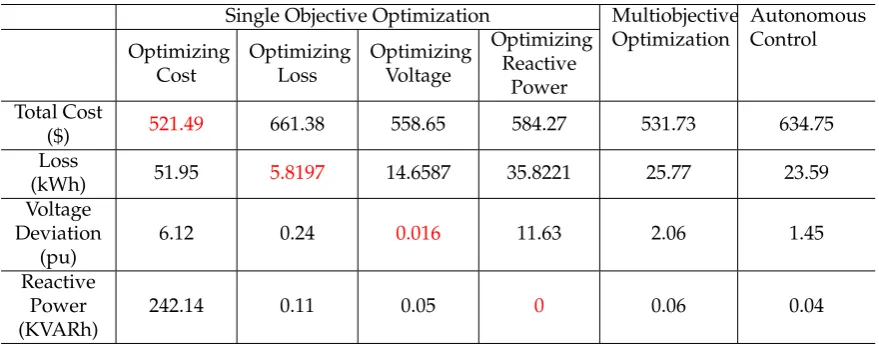
Table 2.Evaluation of solutions of single objective optimization and multiobjective optimization for grid-connected operation
Single Objective Optimization Multiobjective
Optimization
Autonomous Control Optimizing
Cost
Optimizing Loss
Optimizing Voltage
Optimizing Reactive
Power Total Cost
($) 521.49 661.38 558.65 584.27 531.73 634.75
Loss
(kWh) 51.95 5.8197 14.6587 35.8221 25.77 23.59
Voltage Deviation
(pu)
6.12 0.24 0.016 11.63 2.06 1.45
Reactive Power (KVARh)
In order to show the benefit of multiobjective optimization, both single objective optimization problems and a multiobjective optimization problem are solved for grid-connection operation. The solutions, i.e. real and reactive power of DGs and battery are evaluated by calculating the corresponding terms, i.e., total cost, network loss, voltage deviation and total reactive power at PCC. The results are compared in Table2. When the problem is formulated as single objective optimization, the targeted term is always optimized to be the best (as shown in red) compared to that of other solutions (the rest in the same row). By the multiobjective optimization, none of these terms are always the best, but the objectives are optimized together. Network loss is weighted the least based on the AHP process. Nevertheless, all of these solutions are Pareto solutions, i.e., one cannot improve one term without sacrificing another.
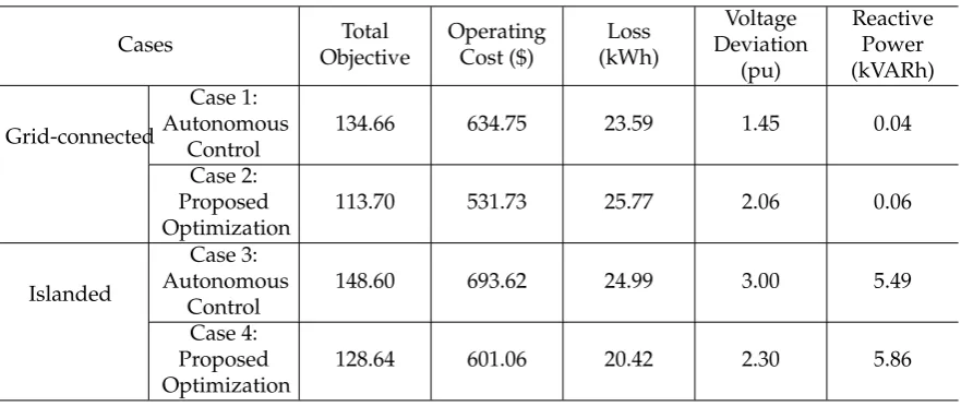
4.2. Comparison of Cost between Different Cases
In order to show the benefit of integrating building thermal dynamics into community microgrid scheduling, we compare the total cost calculated by the proposed optimization and that of autonomous temperature control. In the case of autonomous control, the on/off state of HVAC system can be directly determined by solving equation (5) and performing the logic of temperature controlled relay. Then, the total cost can be calculated by scheduling the same microgrid with predetermined HVAC status. The weighting coefficients are set as: WC=0.2084, WQ=0.1171, WV=0.6116, and WL=0.0629 for all cases. Four cases are studied:
• Case 1: Autonomous temperature control in grid-connected mode • Case 2: Proposed optimization in grid-connected mode
• Case 3: Autonomous temperature control in islanded mode • Case 4: Proposed optimization in islanded mode
Table 3.Costs of the community microgrid in different cases
Cases ObjectiveTotal OperatingCost ($) (kWh)Loss
Voltage Deviation
(pu)
Reactive Power (kVARh)
Grid-connected
Case 1: Autonomous
Control
134.66 634.75 23.59 1.45 0.04
Case 2: Proposed Optimization
113.70 531.73 25.77 2.06 0.06
Islanded
Case 3: Autonomous
Control
148.60 693.62 24.99 3.00 5.49
Case 4: Proposed Optimization
128.64 601.06 20.42 2.30 5.86
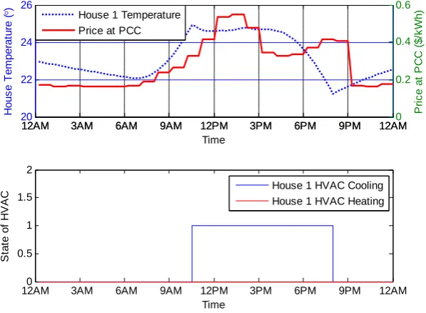
4.3. Operation in Grid-Connected Mode
The results of community microgrid scheduling in grid-connected mode through different
control and optimization methods are compared. Taking house #1 for example, the indoor
temperature and HVAC status are shown in Figure5. Comparing Figure5awith Figure5bclearly shows how the proposed model considering can precool the house to reduce the HVAC consumption during peak price intervals. In specific, by the proposed optimization, the HVAC in house #1 is turned on before 9 AM when the indoor temperature is still comfortable. The house is precooled, so the HVAC can be turned off during the pick price intervals between 1 PM-2 PM.
12AM 3AM 6AM 9AM 12PM 3PM 6PM 9PM 12AM
20 22 24 26 Time H o u s e T e m p e ra tu re (° )
12AM 3AM 6AM 9AM 12PM 3PM 6PM 9PM 12AM0
0.2 0.4 0.6 P ri c e a t P C C ( $ /k W h )
House 1 Temperature Price at PCC
12AM0 3AM 6AM 9AM 12PM 3PM 6PM 9PM 12AM
0.5 1 1.5 2 Time S ta te o f H V A
C House 1 HVAC Cooling
House 1 HVAC Heating
(a)Autonomous temperature control
12AM 3AM 6AM 9AM 12PM 3PM 6PM 9PM 12AM
22 23 24 25 Time H o u s e T e m p e ra tu re (° )
12AM 3AM 6AM 9AM 12PM 3PM 6PM 9PM 12AM0
0.2 0.4 0.6 P ri c e a t P C C ( $ /k W h )
House 1 Temperature Price at PCC
12AM0 3AM 6AM 9AM 12PM 3PM 6PM 9PM 12AM
0.5 1 1.5 2 Time S ta te o f H V A
C House 1 HVAC Cooling
House 1 HVAC Heating
(b)Proposed Optimization
Figure6illustrates how the load is shifted by the proposed optimization comparing with the autonomous control method. As can be expected, the loads are shifted earlier in response to the price. Specifically, loads are shifted before the first price peak, so the second price peak can be avoided. With better thermal insulation of the house, the first price peak can also be avoided.
12AM0 3AM 6AM 9AM 12PM 3PM 6PM 9PM 12AM
50 100 150 200
Time
M
ic
ro
g
ri
d
L
o
a
d
(
k
W
)
Autonomous Control
Proposed Optimization
12AM0 3AM 6AM 9AM 12PM 3PM 6PM 9PM 12AM
0.2 0.4 0.6 0.8
Time
P
ri
c
e
a
t
P
C
C
(
$
/k
W
h
)
Price at PCC
Figure 6.Load shifting in grid-connected mode
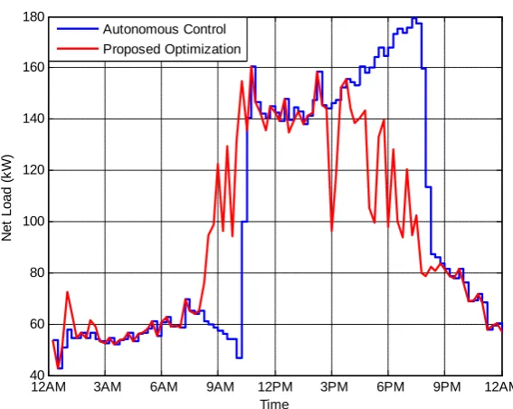
4.4. Operation in Islanded Mode
12AM 3AM 6AM 9AM 12PM 3PM 6PM 9PM 12AM 21 22 23 24 25 Time H o u s e T e m p e ra tu re (° )
12AM 3AM 6AM 9AM 12PM 3PM 6PM 9PM 12AM0
50 100 150 200 T o ta l L o a d ( k W )
House 1 Temperature
Net Load
12AM0 3AM 6AM 9AM 12PM 3PM 6PM 9PM 12AM
0.5 1 1.5 2 Time S ta te o f H V A
C House 1 HVAC Cooling
House 1 HVAC Heating
(a)Autonomous temperature control
12AM 3AM 6AM 9AM 12PM 3PM 6PM 9PM 12AM
22 24 26 Time H o u s e T e m p e ra tu re (° )
12AM 3AM 6AM 9AM 12PM 3PM 6PM 9PM 12AM0
100 200 T o ta l L o a d ( k W )
House 1 Temperature
Total Load
12AM0 3AM 6AM 9AM 12PM 3PM 6PM 9PM 12AM
0.5 1 1.5 2 Time S ta te o f H V A
C House 1 HVAC Cooling
House 1 HVAC Heating
(b)Proposed Optimization
Figure 7.House temperature and HVAC status in islanded mode
12AM 3AM 6AM 9AM 12PM 3PM 6PM 9PM 12AM 40
60 80 100 120 140 160 180
Time
N
e
t
L
o
a
d
(
k
W
)
Autonomous Control
Proposed Optimization
Figure 8.Load shifting in islanded mode
5. Conclusions
In this paper, an MICP-based community microgrid scheduling model considering building thermal dynamics and network operational constraints is proposed. The model directly integrates the detailed thermal dynamic characteristics of buildings into the optimization scheme and enables smart scheduling of HVAC systems. The proposed model optimizes both microgrid operating cost and system performance indices, such as network loss, voltage deviation and power factor at PCC. Numerical simulations on the modified ORNL DECC microgrid show the effectiveness of the proposed model and significant saving in electricity cost can be achieved with network operational constraints satisfied.
Acknowledgments: This work is supported by the U.S. Department of Energy’s Office of Electricity Delivery and Energy Reliability (OE) under Contract No. DE-AC05-00OR22725. This work also made use of Engineering Research Center Shared Facilities supported by the Engineering Research Center Program of the National Science Foundation and the Department of Energy under NSF Award Number EEC-1041877 and the CURENT Industry Partnership Program.
Author Contributions:Guodong Liu carried out the main research tasks and wrote the full manuscript. Thomas B. Ollis and Bailu Xiao participated in the development of the proposed methodology and the literature review. Xiaohu Zhang and Kevin Tomsovic provided important suggestions on writing of the paper.
The authors declare no conflict of interest.
Nomenclature
The main symbols used in this paper are defined below. Others will be defined as required in the text. A bold symbol stands for its corresponding vector or matrix.
Indices and Sets
i Index of DGs, running from 1 toNG.
b Index of batteries, running from 1 toNB.
h Index of houses, running from 1 toNH.
v Index of PV generation, running from 1 toNV.
f Index of feeders, running from 1 toNF.
t Index of time periods, running from 1 toNT.
m Index of energy blocks offered by DGs, running from 1 toNI.
Gn Sets of DGs connected at busn.
Bn Sets of batteries connected at busn.
Hn Sets of houses connected at busn.
Vn Sets of PV connected at busn.
Ω Sets of feeders.
Variables
Binary Variables
uit 1 if DGiis scheduled on during periodtand 0 otherwise.
uCht,uHht 1 if HVAC of househis scheduled cooling/heating during periodtand 0 otherwise.
uCbt,uDbt 1 if batterybis scheduled charging/discharging during periodtand 0 otherwise. Continuous Variables
pit(m) Power output scheduled from them-th block of energy offer by DG i during periodt.
Limited topmaxit (m).
Pit,Qit Real/reactive power output scheduled from DGiduring periodt. PbtC,PbtD Charging/discharging power of batterybduring periodt.
Qbt Reactive power of batterybduring periodt. SOCbt State of charge of batterybduring periodt. PtPCC,QPCCt Real/ reactive power at PCC during periodt.
Pht,Qht Real/reactive load of househduring periodt.
PhtLS,QLSht Real/reactive load curtailment of househduring periodt.
TIn
ht Indoor temperature of househduring periodt.
ThtM The temperature of thermal accumlating layer of inner walls and floor in househduring periodt.
ThtE The temperature of house envelop during periodt.
Vnt Voltage magnitude of busnduring periodt.
Pf t,Qf t Real/ reactive power flow on line f during periodt. lf t Squared amplitudes of current on linef during periodt. Constants
λit(m) Marginal cost of them-th block of energy offer by DGiduring periodt.
λPCCt Purchasing price of energy from distribution grid during periodt.
Cbt Degradation cost of batterybduring periodt. VhtLS Cost of load curtailment of househduring periodt.
Pmax
i ,Pimin Maximum/minimum output of DGi. PPCC,max Maximum input/output power at PCC.
Pvt,Qvt Real/reactive power output from PVvduring periodt.
PhtO,QOht Real/reactive power consumption scheduled for non-HVAC load in house h during periodt.
PhH Rated power of HVAC system in househ.
PbC,max,PbD,max Maximum charging/discharging power of batteryb.
SOCbtmax,SOCbtmin Maximum/minimum state of charge of batterybduring periodt.
PhtLS,max Maximum load curtailment of househduring periodt. ηCb,ηDb Battery charging/discharging efficiency.
ωht Customer discomfort cost of househduring periodt. δht Allowed temperature deviation of househduring periodt.
ThtD Desired indoor temperature of househduring periodt. Φt Solar irradiance during periodt.
RA
h Thermal resistance between room air and ambient of househ.
RMh Thermal resistance between room air and the thermal accumulating layer in the inner walls and floor of househ.
REh Thermal resistance between room air and the envelope of househ.
REA
h Thermal resistance between the envelope of househand the ambient. CInh Total thermal capacitance of the indoor air of househ.
CMh Total thermal capacitance of the inner walls of househ.
CEh Total thermal capacitance of the house envelope of househ.
psh The fraction of solar radiation entering the inner walls and floor of househ, then the rest of the solar energy is absorbed by the indoor air.
ηh Coefficient of performance (COP) of HVAC in househ.
Vthrmax,Vthrmin Maximum/Minimum voltage thresholds beyond which voltage deviation will be minimized.
Vmax,Vmin Maximum/Minimum voltage deviations.
Si,Sb,Sf Apparent power limit of DGi, batteryband line f. rf,xf resistance and reactance of line f.
Imaxf Maximum amplitudes of current on linef. tan(θi) Power factor limit of DGi.
tan(θC
b), tan(θDb) Power factor limits of batterybwhen charging/discharging.
tan(θPCC,max) Power factor limits of PCC.
tan ϕHh, tan ϕOh Power factor of HVAC and non-HVAC load at househ.
Bibliography
1. Lasseter, R.; Akhil, A.; Marnay, C.; Stephens, J; Dagle, J.; Guttromson, R.; Meliopoulous, A.S.; Yinger, R.; Eto, J. CERTS Microgrid Concept, April 2002. Available online: https://pserc.wisc.edu/documents/research_documents/certs_documents/certs_publications/certs_micro grid/certsmicrogridwhitepaper.pdf(accessed 15, August 2017).
2. Madureira A.G.; Pecas Lopes, J.A. Coordinated voltage support in distribution networks with distributed generation and microgrids.IET Renew. Power Gen.2009,3, 439-454.
3. Beer, S.; Gomez, T.; Dallinger, D.; Momber, I,; Marnay, C.; Stadler, C. An economic analysis of used electric vehicle batteries integrated into commercial building microgrids.IEEE Trans. Smart Grid2012,3, 517-525. 4. Tsikalakis, A.G.; Hatziargyriou, N.D. Centralized control for optimizing microgrids operation.IEEE Trans.
Energy Convers.2008,23, 241-248.
5. Agrawal, M.; Mittal, A. Microgrid technological activities across the globe: A review.Int. J. Res. Rev. Appl. Sci.2011,7, 147-152.
6. Gu, W.; Wu, Z.; Bo, R.; Liu, W.; Zhou, G.; Chen, W.; Wu, Z.; Modeling, planning and optimal energy management of combined cooling, heating and power microgrid: A review.Int. J. Electr. Power Energy Syst. 2014,54, 26-37.
7. Belvedere, B.; Bianchi, M.; Borghetti, A.; Nucci, C.A.; Paolone, M.; Peretto, A. A microcontroller-based power management system for standalone microgrids with hybrid power supply. IEEE Trans. Sustain. Energy2012,3, 422-431.
8. Morais, H.; Kadar, P.; Faria, P.; Vale, Z.A.; Khodr, H.M. Optimal scheduling of a renewable micro-grid in an isolated load area using mixed-integer linear programming.Renew. Energy2010,35, 151-156.
9. Babazadeh, H.; Gao, W.; Wu, Z.; Li, Y. Optimal energy management of wind power generation system in islanded microgrid system. In Proceedings of the North American Power Symposium(NAPS), Manhattan, Kansas, USA, 22-24 September 2013.
10. Palma-Behnke, R.; Benavides, C.; Lanas F.; Severino, B.; Reyes, L.; Llanos, J.; Saez, D. A microgrid energy management system based on the rolling horizon strategy.IEEE Trans. Smart Grid2013,4, 996-1006. 11. Sobu, A.; Wu, G. Dynamic optimal schedule management method for microgrid system considering
12. Mohamed, F.A.; Koivo, H.N. System modelling and online optimal management of MicroGrid using Mesh Adaptive Direct Search.Int. J. Electr. Power Energy Syst.2010,32, 398-407.
13. Cardoso, G.; Stadler, M.; Siddiqui, A.; Marnay, C,; DeFrost, N.; Barbosa-Povoa, A.; Ferrao, P. Microgrid reliability modeling and battery scheduling using stochastic linear programming. Electr. Power Syst. Res. 2013,103, 61-69.
14. Nguyen, D.T.; Le, L.B. Optimal Bidding Strategy for Microgrids Considering Renewable Energy and Building Thermal Dynamics.IEEE Trans. Smart Grid2014,5, 1608-1620.
15. Liu, G.; Xu, Y.; Tomsovic, K. Bidding Strategy for Microgrid in Day-Ahead Market Based on Hybrid Stochastic/Robust Optimization.IEEE Trans. Smart Grid2016,7, 227-237.
16. Daratha, N.; Das, B.; Sharma, J. Coordination Between OLTC and SVC for Voltage Regulation in Unbalanced Distribution System Distributed Generation.IEEE Trans. Power Syst.2014,29, 289-299. 17. Dolan, M.J.; Davidson, E.M.; Kockar, I.; Ault, G.W.; McArthur, S. Distribution Power Flow Management
Utilizing an Online Optimal Power Flow Technique.IEEE Trans. Power Syst.2012,27, 790-799.
18. Paudyal, S.; Canizares, C.A.; Bhattacharya, K. Optimal Operation of Distribution Feeders in Smart Grids. IEEE Trans. Ind. Electron.2011,58, 4495-4503.
19. Borghetti, A.; Bosetti, M.; Grillo, S.; Massucco, S.; Nucci, C.; Paolone, M.; Silvestro, F. Short-term scheduling and control of active distribution systems with high penetration of renewable resources.IEEE Syst. J.2010, 4, 313-322.
20. Zhou, Q.; Bialek, J. Generation curtailment to manage voltage constraints in distribution networks. IET Gener., Transm., Distrib.2007,1, 492-498.
21. Calderaro, V.; Conio, G.; Galdi, V,; Massa, G.; Piccolo, A. Optimal Decentralized Voltage Control for Distribution Systems With Inverter-Based Distributed Generators.IEEE Trans. Power Syst.2014,29, 230-241. 22. Liu, G.; Ceylan, O.; Xu, Y.; Tomsovic, K. Optimal Voltage Regulation for Unbalanced Distribution Networks Considering Distributed Energy Resources. In Proceedings of the IEEE Power & Energy Society General Meeting (PESGM), Denver, Colorado, USA, 26-30 July 2015
23. Liu, G.; Xu, Y.; Ceylan, O.; Tomsovic, K. A new linearization method of unbalanced electrical distribution networks. In Proceedings of the North American Power Symposium(NAPS), Pullman, Washington, USA, 7-9 September 2014.
24. Shekari, T.; Golshannavaz, S,; Aminifar, F. Techno-Economic Collaboration of PEV Fleets in Energy Management of Microgrids.IEEE Trans. Power Syst.2017,32, 3833-3841.
25. Trakas, D.; Hatziargyriou, N. Optimal Distribution System Operation for Enhancing Resilience Against WildfiresIEEE Trans. Power Syst.2017,99, 1-1.
26. Lavaei, J.; Low, S.H. Zero Duality Gap in Optimal Power Flow Problem. IEEE Trans. Power Syst.2012,27, 92-107.
27. Jabr, R. Radial distribution load flow using conic programming.IEEE Trans. Power Syst.2006,21, 1458-1459. 28. Baran, M.; Wu, F. Optimal capacitor placement on radial distribution systems.IEEE Trans. Power Syst.1989,
4, 725-734.
29. Farivar, M.; Low, S. Branch flow model: Relaxations and convexification —Part I.IEEE Trans. Power Syst. 2013,28, 2554-2564.
30. Nguyen D.T.; Le, L.B. Joint optimization of electric vehicle and home energy scheduling considering user comfort preference.IEEE Trans. Smart Grid2014,5, 188-199.
31. Nguyen D.T.; Le, L.B. Optimal Bidding Strategy for Microgrids Considering Renewable Energy and Building Thermal Dynamics.IEEE Trans. Smart Grid2014,5, 1608-1620.
32. Saaty, T. Decision making-The analytic hierarchy and network processes (AHP/Anp).J. Syst. Sci. Syst. Eng. 2004,13, 1-35.
33. Thavlov, A. Dynamic optimization of power consumption. M.S. thesis, Tech. Univ. Denmark, Kongens Lyngby, Denmark, 2008.
34. Madsen, H.; Holst, J. Estimation of continuous-time models for the heat dynamics of a building. Energy Buildings1995,22, 67-79.
35. Bacher, P.; Madsen, H. Identifying suitable models for the heat dynamics of buildings. Energy Buildings 2011,43, 1511-1522.
37. Taylor, J.A.; Hover, F.S. Conic AC transmission system planning.IEEE Trans. Power Syst.2013,28, 952-959. 38. Baradar, M.; Hesamzadeh, M.R.; Ghandhari, M. Second-order cone programming for optimal power flow
in vsc-type ac-dc grids.IEEE Trans. Power Syst.2013,28, 4282-4291.
39. Carrion, M.; Arroyo, J.M. A computationally efficient mixed-integer linear formulation for the thermal unit commitment problem.IEEE Trans. Power Syst.2006,21, 1371-1378.