http://www.sciencepublishinggroup.com/j/dmath doi: 10.11648/j.dmath.20190401.14
ISSN: 2578-9244 (Print); ISSN: 2578-9252 (Online)
Performance Comparison of Various Kernels of Support
Vector Regression for Predicting Option Price
Biplab Madhu, Arindam Kumar Paul, Raju Roy
Department of Mathematics, Khulna University, Khulna, Bangladesh
Email address:
To cite this article:
Biplab Madhu, Arindam Kumar Paul, Raju Roy. Performance Comparison of Various Kernels of Support Vector Regression for Predicting Option Price. International Journal of Discrete Mathematics. Vol. 4, No. 1, 2019, pp. 21-31. doi: 10.11648/j.dmath.20190401.14
Received: February 6, 2019; Accepted: March 18, 2019; Published: April 10, 2019
Abstract:
The famous Black Scholes Option Pricing Model is a well-known option pricing model. Owing to some limitations it fails to perfectly detect the option price. In this study various regression and optimization techniques for predicting option price and analyzing various phenomena and properties with machine learning techniques for valuation and improving the accuracy of the option pricing model are used. The Proposed method is divided with different stages. Firstly, Principal Component Analysis (PCA) is used in order to identify the most influential inputs in the framework of the option pricing model and to reduce the dimensionality of our working data. Secondly, Support vector machine (SVM) and support vector regression (SVR) is used which is a very special type of learning algorithms characterized by the capacity of input variable as option price parameter and the use of the kernel functions. The combination of these two methods shows that SVM and PCA can perform better by consuming less time and memory. In this study, we investigate the estimation performance of option pricing model with SVM and PCA. A brief analysis of the accuracy of the approach also provided. The training of SVM and normalization of PCA is computed by MATLAB and it leads towards a new way for predicting option price perfectly if the formulation will be simulated using enough data.Keywords:
Support Vector Regression, Gaussian Process, Financial Data Modeling and Forecasting, Option Price, Principal Component Analysis1. Introduction
Now a day one of the most important topics in finance is the valuation of option pricing. Option price accuracy yet difficult task in computational financial world. It follows a complex pattern and a stochastic behavior in stock price. ‘Option’ which is the right (not the obligation) to buy (call option) or sell (put option) the underlying asset at a particular price. Options can reduce the financial risk on the future events [12]. Since 1970 many methods were adopted for dealing this type of problem. The influential work in the field of option pricing is done by Black and Scholes (1973) with their formula for option pricing or more famously known as the Black-Scholes equation for Option Pricing [2]. It is difficult to justify certain assumptions for different parametric specification in the real-world data as there exists nonlinear relationship between option price and various variables. Therefore, in recent years, many researchers turned in to machine learning or nonparametric methods as they are
capable to capture nonlinear relationship between input and output [2, 14].
Two different approaches will be given in this study. The first approach is using Principal Component Analysis (PCA) was invented by Karl Pearson (1901). Principal Component Analysis is considered an experimental technique that can be used to gain a better understanding of the interrelationships between variables. Principal Component Analysis (PCA) can be consumed to test for normalcy. In this study the Principal Component Analysis (PCA) used to Normalize the original data to a simple data.
The other approach is using Support Vector Machine (SVM). One of the objectives of financial methods is price of option evaluation. In this study, it is concentrated more on the Support Vector Machine, a pattern classification algorithm was developed by V. Vapnik (1992). Support Vector Regression (SVR) and Support Vector Machine are powerful methodology for approximating complex function.
PCA and SVM to predict option prices. In these approaches, the PCA serves as a state estimator and makes predictions based on the Black-Scholes formula. The residuals between the actual prices and the Black-Scholes model are fed into the SVM in the model, and the SVM is conducted to further reduce the prediction errors. Empirical results of this study established that the model of PCA and Support Vector Machine. The empirical results shown that the PCA can capture all of the patterns in the option prices, and the performance of the model can significantly reduce the option price errors.
2. Related Work
A large number of academic studies have examined the relative performance of options price in several countries, few of the studies are mentioned here. Hutchinson et al. [14] in 1994 used neural network for option pricing and compared its performance with Black Scholes model. The proposed model performed fairly well. M. Liu [22] in 1996, Yao et al. [31] in 2000 and Andreou [1] in 2008 successfully applied neural network in option pricing. Saxena [26] studied European-style CNX Nifty Options traded at National Stock Exchange of India. He combined the BS model and Artificial Neural Networks (ANNs), for option pricing and concluded that hybrid model can improve the pricing performance of options under all market conditions and Mitra [23] in 2012 studied Nifty Options in India and forecasted it using neural network. Lajbcygier et al. [19] improved the Hybrid Neural Network using bootstrap methods to reduce bias in existing model.
There are so many researches, in which Support Vector Regression has been successfully used as option pricing tool. In my previous work Support Vector Regression and multiple kernel Support Vector Regression has been successfully used for nifty index option pricing. M. M. Pires et al [24] compared the performance of a Multi-Layer Perceptron neural network and a Support Vector Regression in pricing American styled options. It was concluded that a Support Vector Regression approach provided promising results than that found with Multi-Layer Perceptron. S. C. Huang et al. [13] combined the unscented Kalman filters (UKFs) and Support Vector Regression (SVR) to predicting option prices. The difference between the market option prices and the Black-Scholes option price is taken input to SVR for reducing the prediction errors. The performance of the new hybrid model is better than pure SVR models or UKFs models in option pricing. P. Wang et al. [30] used Support Vector Regression (SVR) integrated with stochastic volatility models for forecasting of currency option pricing. The results reveal that integrated model performed better than traditional approaches such as Garman-Kohlhagen Formula (GK) model and ANN Option pricing model. Panayiotis C. Andreou et.al. [1] used Support Vector Regression and Least Squares Support Vector Regression for pricing S&P 500 index call options with Deterministic Volatility Functions approach and compared results with the traditional Black Scholes model.
He obtained promising results for the both SVR models. L. Xun, et al. [21] gave some modifications on three parametric methods, the binomial tree method, the finite difference method and the Monte Carlo method, to forecast the option prices and further refined the forecast results by nonparametric methods ANN and SVR by decreasing the nonlinear errors. He found that, compared with the standard and improved parametric option price forecasting methods, the ANN and SVR have higher forecasting accuracy. ChihMing Hsu et al. [13] compared the price of Taiwan Stock Exchange Capitalization Weighted Stock Index Options (TAIEX Options) by three approaches i.e. Black-Scholes (BS) model, Genetic Programming (GP) and Support Vector Regression (SVR) with all basic factors in the B-S model and the other factors in GP and SVR model. They concluded that, both GP and SVR forecasting models gave more promising results than Black-Scholes model.
For further improving forecasting performance in option pricing, multiple kernel Support Vector Regression with SMO algorithm is applied. There are many kernel methods which have been applied in various applications, Multiple Kernel Learning is one of them, where kernels are combined in linear or nonlinear ways for maximizing a generalized performance. This approach learns both Lagrange’s multipliers and kernel weights in a single optimization Lanckriet et al. [20]. In the area of kernel learning F. R. Bach et al. [3] considered combinations of kernel matrices in MKL based on sequential minimization optimization with smoothed version of the given problem.
In this paper the Principal component analysis (PCA) is used to normalized the data, Support vector machine (SVM) and SVR with various kernel are applying to predict the option price. The paper is structured as follows. First introduce the theoretical analysis of Black-Scholes, Principal Component analysis (PCA), Support vector machine (SVM) and Support vector regression (SVR). In second, this report discusses about the data structure and algorithm on each type of option pricing dataset. Then result and discussion with scope and limitations is described and Conclusion is presented in last section.
3. Related Literature Reviews
This section provides related topics that were used to
create the proposed system. Black- Scholes Model (BS),
Principalcomponentanalysis(PCA),Supportvectormachine
(SVM)andSupportvectorregression(SVR)areexplainedin
short.
3.1. Black-Scholes Option Pricing Model
The Black-Scholes Model describes the behavior of options on assets that follow a Geometric Brownian Motion that satisfies the following stochastic differential equation
. .
dS=µS dt+σS dX , or dS dt dX
Where,µ = drift rate: The mean change per unit time for a stochastic process is known as the drift rate, σ= standard deviation: The variance per unit time is known as the
variance rate, X = standard Brownian motion,S= Current
stock price, t= unit time
The variable µ is the stock’s expected rate of return. The
variableσis the volatility of the stock price. The variable σ2 is referred to as its variance rate. The model in the above equation represents the stock price process in the real world. In a risk-neutral world, µequals the risk-free rate r. This model is often referred to as the geometric Brownian motion assumption in Black-Scholes, which looks like geometric growth driven by a drifting Brownian motion. In this paper, beside these parameter it also use the parameter Rho (ρ ), Gamma (Γ), Vega (Λ) to predict the option price of a data set.
3.2. Principal Component Analysis (PCA)
One of the main problems in statistics is the problem of picturing data that has many variables. But when there are more than three variables, it is more complex to imagine their connections. In data sets there are many variables, groups of
variables often change together. In many systems there are only a few such dynamic forces. But a plenty of planning enables us to measure dozens of system variables. This report can simplify the problem by substituting a group of variables with a single new variable.
Principal component analysis (PCA) is a quantitatively challenging method for achieving this simplification. The method produces a new set of variables, called principal components. Each principal component is a linear combination of the original variables. Every principal component is orthogonal to each other. The principal components as a whole form an orthogonal basis for the area of the data. From the above discussion the full set of principal components is as large as the original set of variables. But it is common for the sum of the variances of the first few principal components to exceed 80% of the total variance of the original data. To use PCA, it needs to have the actual measured data that is to be analyzed. However, if it has shortage the actual data, but have the sample covariance or correlation matrix for the data. To reduce the dimension of our original data by PCA, the following methodology is use.
Support vector machine (SVM) and Support vector regression (SVR).
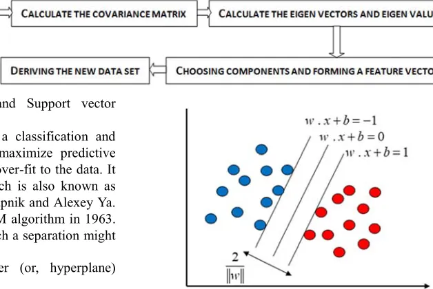
Support Vector Machine (SVM) is a classification and regression forecast tool that uses to maximize predictive accuracy while automatically avoiding over-fit to the data. It is a supervised learning algorithm which is also known as Support vector network. Vladimir N. Vapnik and Alexey Ya. Chervonenkis invented the original SVM algorithm in 1963. Depending on the nature of the data, such a separation might be linear or non-linear.
Let us consider a linear classifier (or, hyperplane) ( ) T
f x =w x+b
where wrepresents weight vector, x is the input feature vector and b represents the position of the hyperplane. Here,
(a)if the input vector is 2-dimensional, the linear equation will represent a straight line.
(b)if the input vector is 3-dimensional, the linear equation will represent a plane.
(c)if input vector more than 3-dimension, the linear equation will represent a hyperplane.
The SVM algorithm is to find an optimal hyperplane for classification of two classes. Assume that the equation of hyperplane is wT
x
+ =b 0. The distance between w.x
+ = +b 1 and w.x
+ = −b 1is the margin of this hyperplane. By applying the distance rule between two straight lines, we get themargin, m 2
w
=
Figure 1. Maximum margin hyperplanes for SVM trained with samples with classes.
For non-linear classifier SVM use kernel function to separate the data points. Obtain a nonlinear SVM regression model by replacing the dot product x1T.x2 with a nonlinear kernel function K x x( 1, 2)=<ϕ(x1), (ϕ x2)> where, ϕ( )x is a
transformation that maps x to a high-dimensional space.
Popular kernel functions are
a Linear kernel function: K x( j,xk)=xjTxk
b Gaussian kernel function: K x( j,xk)=exp(− xj−xk 2)
c Polynomial kernel function: K x( j,xk)= +(1 xjTxk)q
where xi and xj are support vector where support vector is
Simply, support vectors are the data points that lie closest to the decision surface (or hyperplane).
4. Data Structure and Methodology
Financial data offer an excellent source of difficult and challenging problems to the computing community. Many applications, time series prediction to stock selection have been attempted. Hutchinson et. al. (1994) and Niranjan (1996), focused on the widely used Black-Scholes formula may be obtained with neural networks, while the latter looked at the non-stationary aspects of the problem. De Freitas et. al. extends this work by incorporating noise
estimation and powerful sampling algorithms. In this section, it will present some useful discussion. Firstly, it discusses the data structure and source of the data. Then discussion about the relationship between predictor and response of the data. The next section will discuss the accuracy of the given data using SVM and PCA method. Finally, it will observe the accuracy of the predicted option prices.
We collect the data from the spy option of yahoo finance 2015. From this data, we will calculate the accuracy of the option price. In the original data, we modified some of the dimensions of the variable.
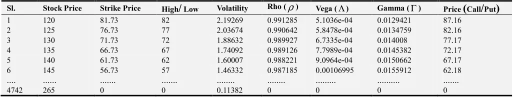
Table 1. Optionpricedataofmarketvalue.
Sl. Stock Price Strike Price High
/
Low Volatility Rho ( ) Vega ( ) Gamma ( ) Price(
Call/
Put)
1 120 81.73 82 2.19269 0.991285 5.1036e-04 0.0129421 87.162 125 76.73 77 2.03674 0.990642 5.8478e-04 0.0134759 82.16 3 130 71.73 72 1.88632 0.989927 6.7335e-04 0.014008 77.17 4 135 66.73 67 1.74092 0.989126 7.7989e-04 0.0145382 72.17 5 140 61.73 62 1.60007 0.988221 9.0964e-04 0.0150662 67.17 6 145 56.73 57 1.46332 0.987185 0.00106995 0.0155912 62.18
.... ... ... ... ... ... ... ... ...
4742 265 0 0 0.11382 0 0 0 0
4.1. First Approach
Firstly, this paper evaluated and tested the relationship between input variables and output variables by using a simple quadratic polynomial regression after standardizing the data by its mean and standard deviation and by transforming the data with the bi-square weighting scheme. This paper calculated various measurements which are discussed below.
4.1.1. What is R-Squared
R-squared is a statistical measure of how close the data are to the fitted regression line. It is also known as the coefficient of determination, or the coefficient of multiple determination for multiple regression. The definition of R-squared is fairly a straight-forward; it is the percentage of the response variable variation that is explained by a linear model, or
a R-squared = Explained variation / Total variation
b R-squared is always between 0 and 100%:
c 0% indicates that the model explains none of the
variability of the response data around its mean.
d 100% indicates that the model explains all the
variability of the response data around its mean. In general, the higher the R-squared, the better the model fits data. The adjusted R-squared compares the explanatory power of regression models that contain different numbers of predictors. The adjusted R-squared is a modified version of R-squared that has been adjusted for the number of predictors in the model. The adjusted R-squared increases only if the new term improves the model more than would be expected by chance. It decreases when a predictor improves the model by less than expected by chance. The adjusted R-squared can be negative, but it’s usually not. It is always lower than the R-squared.
4.1.2. How to Increase R-squared and Adjusted R-squared
Since our data is a bit noisy and not scaled for training a
machine learning model. It had seen that data is unable to fit a 3rd degree polynomial model. So, it’s necessary to normalize our dataset. From above discussion, the value of data is not suitable and there is a very weak relationship among them, so there are a few options for removing this limitation.
a Removing residuals
b Removing Outliers
c Normalizing and Scaling Data so that it can fit a model
An alternative weighting scheme is to weight the residuals using a bi-square. This stage, first compute the residuals from the unweighted fit and then apply the following weight function:
( )
22
( ) 1
6
X W X
M
= −
where, M is the median absolute deviation of the residuals. The weight is set to 0 if the absolute value of the residual is
greater than 6M . This method provides an effective
alternative to deleting specific points. Extreme outliers are deleted, but mild outliers are reweighted rather than deleted altogether. The values of R-squared and Adjusted R-squared after applying this method are:
4.2. Second Approach
Table 2. OptionpricevsparameterwithRegression.
Data Description R Squared Adjusted R Squared Ask price Vs Price 0.387371753 0.38698385 Bid price Vs Price 0.392074849 0.391689924 Delta vs Price 0.231357145 0.230870456 Implied Volatility Vs Price 0.08705332 0.086475262 Risk-Free interest rate Vs Price 0.014252846 0.012795256 Strike Price vs Price 0.081934017 0.081352717 Vega Vs Price 0.022020475 0.020574371
4.2.1. Evaluating theModel UsingSVM and PCA
In the market price data, this paper takes the seven-input variable. But the Table 1, we see that there are 4742 rows of data with respect to these seven input Variables. The Required Input and the output Variables are:
Stock Price
Strike Price
High/ Low
Volatili ty
Rho ( )
Vega ( )
Gamma ( )
Price (Call/ Put)
But in the above data table, the 4742 rows and eight columns are difficult to run the data into any program. So, we use the PCA to normalize the data. By using the PCA the normalization of the seven column is transformed into two columns. By this time the 4742 rows and the two columns are eligible to run the programmer for valuation of the option price. The required two input variables able to explain 68.6% and 33.3% of Variance of the total data are:
Var Name 1 Var Name 2
Feasibility gap obtained by SMO is a nonnegative scalar. If Gap Tolerance is 0, then SVM does not use this parameter to check convergence. The reason behind the convergence is Feasibility gap in our case. The Feasibility gap found after converging is mentioned the Table 2 Here we have experimented three different types of kernels for evaluating the actual phenomena and explaining the behavior of the data. After testing the SVM model with Quadratic Kernel with 4 Principle Component, we have experimented the same data with
a Quadratic Kernel with 2 Principle Component
b Gaussian Kernel and 2 Principle Component
c Gaussian Kernel and 2 Principle Component (Highly
Optimized)
Now the performance of a Support Vector Regression Model can be measured with its parameters and number of
Support Vector points. We have summarized all together
below:
Table 2. MeasurementofSVRwiththevariouskernel.
SVR with Various Kernel Measurements
Quadratic Kernel with 2 Principle Components
Gaussian Kernel and 2 Principle Components
Gaussian Kernel and 2 Principle Components (Highly Optimized)
Support Vector Points 4386 2354 4656
Epsilon (
ε
) 0.002 0.2 0.002Iterations 142001 1665 3527
Bias 18.03 -18.60 13.60
Box Constraints 40 40 80
DeltaGradient 1.99 0.28 0.28
RMSE 19.59 21.18 18.43
R-Squared 0.25 0.27 0.36
Gap 9.1913e-04 4.004e-04 8.242e-04
5. Discussion
Figure 2. Identified Pattern by SVR with Quadratic Kernel Where Epsilon (
ε
) = 0.002.Figure 2 shows that the prediction of pattern with real option price. This figure, shows that the real option price and the predicted pattern is far away. These blue points refer to the real option price and the red points refer to predicted patterns. In this figure, the value of R-Squared is 0.25. So, the quadratic kernel with Predicted price and real option
price is covered by these patterns.
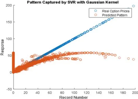
Figure 3 shows that the prediction of pattern with real option price with Gaussian kernel. This figure, shows that the real option price and the predicted pattern is nearly close to each other comparing with Quadratic kernel pattern. These blue points refer to the real option price and the red points refer to predicted patterns. In this figure, the value of R-Squared is 0.27.
Figure 3. Identified Pattern by SVR with Less Optimized Gaussian Kernel Where Epsilon (ε ) = 0.2.
Figure 4 shows that the prediction of pattern with real
option price. This figure, shows that the real option price and the predicted pattern is nearly close to each other comparing with the Quadratic kernel and Gaussian kernel pattern. These blue points refer to the real option price and the red points refer to predicted patterns. So, the Gaussian kernel (with highly optimized) with Predicted price and real option price is maximally covered by these patterns.
Figure 4. Identified Pattern by SVR with Highly Optimized Gaussian Kernel Where Epsilon (ε) = 0.002.
Figure 5 shows that the response of the pattern with the record number. This figure, shows that the actual option price and the predicted option price by SVR with the Quadratic kernel. These blue points refer to the predicted option price and the red points refer to the actual option price. This figure, shows that with Quadratic kernel the actual option price and the predicted option price maximally covered.
Figure 5. Response Plot of Quadratic SVR.
Figure 6. Logarithmic Response Plot of Quadratic SVR.
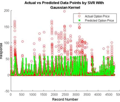
Figure 7. Response Plot of Gaussian SVR.
Figure 7 shows the response of the pattern with the record number. This figure, shows that the actual option price and the predicted option price by SVR with the Gaussian kernel. These blue points refer to the predicted option price and the red points refers to the actual option price. This figure, shows that with Gaussian kernel the actual option price and the predicted option price mostly covered. For this pattern the number if iteration is 1665.
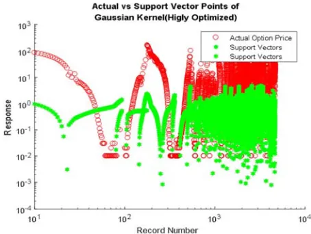
Figure 9. Response Plot of Gaussian SVR (Highly Optimized).
Figure 9 shows that the response of the pattern with the record number. This figure, shows that the actual option price and the predicted option price by SVR with Gaussian kernel (Highly Optimized). These blue points refer to the predicted option price and the red points refers to the actual option price. This figure, shows that with Gaussian kernel (Highly Optimized) the actual option price and the predicted option price are maximumly covered comparing with the Quadratic and Gaussian kernel. Here the number of iterations is 3527. The bias also positive. So, the Gaussian kernel (Highly Optimized) best kernel among the above three kernels.
Figure 10. Logarithmic Response Plot of Gaussian SVR (Highly Optimized).
Figure 11. Support vector of SVR with Quadratic Kernel.
Figure 12. Logarithmic Support vector of SVR with Quadratic Kernel.
Figure 11 shows the price of the pattern with record the number. This figure, shows that the actual data points and the support vector points by SVR with the Quadratic kernel. These blue points refer to the actual data points and the red points refers to the support vector points. This figure, shows that with Quadratic kernel the support vector can capture 4386 points. Where the box constraint is 40.
Figure 13. Support vector of SVR with Gaussian Kernel.
Figure 13 shows that the price of the pattern with the record number. This figure, shows that the actual data points and the support vector points by SVR with Gaussian kernel. These blue points refer to the actual data points and the red points refer to the support vector points. This figure, shows that with Gaussian kernel the support vector can capture 2354 points. Where the box constraint is 40. So that comparing with the Quadratic kernel, the Gaussian kernel can capture fewer vector points.
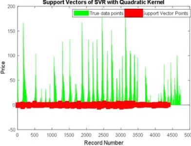
Figure 15. Support vector of SVR with Highly Optimized Gaussian Kernel.
Figure 15 shows that the price of the pattern with the record number. This figure, shows that the actual data points and the support vector points by SVR with Gaussian kernel (Highly Optimized). These blue points refer to the actual data points and the red points refer to the support vector points. This figure, shows that with Gaussian kernel (Highly
Optimized) the support vector can capture 4656 points. Where the box constraint is 8. So that comparing with the Quadratic kernel and Gaussian kernel the Gaussian kernel (Highly Optimized) can capture the most vector points.
Figure 16. Logarithmic Support vector of SVR with Highly Optimized Gaussian Kernel.
Now in the below, this section describes a table comparing with the Quadratic Kernel SVR, Gaussian Kernel SVR and Gaussian Kernel (Highly Optimized). In this table, we compute the actual option price and the predicted price with respect to the above three kernels. Among these three kernels the Gaussian kernel (Highly Optimized) the actual option price and the predicted option price is close.
Table 4. PredictionofData.
Quadratic SVR Gaussian SVR (Highly Optimized) Gaussian SVR
Actual Option Price Predicted Option Price Actual Option Price Predicted Option Price Actual Option Price Predicted Option Price
7.00 6.00 7.57 7.80 48.23 34.13332
5.99 5.57 8.40 7.37 40.25 31.72123
6.36 5.20 7.10 6.94 29.99 29.83001
5.83 4.83 6.61 6.53 39.94 29.35138
5.43 4.47 5.98 6.12 35.3 28.94538
5.00 4.16 5.57 5.72 38.15 28.44017
4.74 3.80 5.17 5.32 34.44 27.89789
4.02 3.45 4.82 4.97 36.05 27.38807
3.73 3.12 4.40 4.57 33.4 26.99696
3.20 2.80 4.00 4.20 35.25 26.5183
2.80 2.47 3.64 3.82 33.65 25.95045
2.75 2.20 3.32 3.47 33.23 25.57937
2.12 1.91 2.95 3.12 29.7 24.6109
1.85 1.64 2.58 2.79 28.4 22.20046
1.50 1.39 2.37 2.47 23.55 19.97052
1.30 1.17 2.01 2.17 20.1 17.84221
1.03 0.97 1.75 1.87 17.73 15.57276
0.80 0.78 1.53 1.61 15.85 13.47057
0.60 0.62 1.26 1.36 12.72 11.59791
0.46 0.49 1.03 1.13 11 10.01698
We can see that the SVR with Gaussian kernel scores highest but its support vector points are minimum, And SVR with Quadratic Kernel and another Gaussian Kernel with different epsilon have more support vector points but the
error and R-Squared are less than the middle one. From the above table we can reach the decision that:
a Option prices follow the Gaussian process mostly but if
pattern is as same as the Quadratic SVR.
b The Quadratic SVM can predict option price sometimes
more accurately than Gaussian SVR but R-Squared is low here that indicates more optimization is required for gaining better accuracy. But the SVR with the Quadratic kernel is able to predict those values more accurately.
c If we decrease the value of epsilon, then support vector
points increase highly and it indicates that the model with a smaller margin is highly optimized and able to explain a higher variance.
d It’s possible to predict the option prices which is less than 50 with a high accuracy by using each and every model.
e The larger value of Box Constraints allows us to predict
relatively higher option prices but the accuracy gained it is not satisfactory.
f The training time is very high in case if Quadratic SVR
even after doing PCA.
g Any SVR with Gaussian Kernel is capable to capture
the pattern easily but with low accuracy for each data points but Quadratic SVR is able to capture the partial pattern with a high accuracy.
h After optimizing the SVR with Gaussian Kernel, it
performs like an SVR with Quadratic Kernel and in addition, it is able to predict higher option prices.
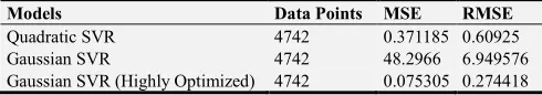
Table 5. PerformanceofvariousSVRinoptionprice.
Models Data Points MSE RMSE Quadratic SVR 4742 0.371185 0.60925 Gaussian SVR 4742 48.2966 6.949576 Gaussian SVR (Highly Optimized) 4742 0.075305 0.274418
6. Scopes and Limitations
a A very small dataset is used here for doing this project
which isn’t enough to capture the pattern of option price and predict them. But for the limited computational capacity, we were unable to work with a bigger dataset. b We didn’t filter the data which may bring significant
change in this case.
c We think that adding more input variables like the
difference between two successive option prices can be included for tuning the model and for gaining better accuracy.
d This paper's aim was to apply various mathematical
techniques like Linear Programming, Control,
Optimization and etc. than only learning pattern from the data. If it’s possible to access better research environment with highly configured machines, this work can be extended towards an automated software which can continuously predict option prices.
7. Conclusion
In this report, we study the use of Support Vector Machines (SVM) and Principal Component Analysis (PCA)
to analyze the option price. The estimator is based on the Black-Scholes Model, which is captured by the SVR and PCA. Compared with another hybrid model based on SVR and PCA. In any case, PCA and SVR is a successful system to understand minimization. SVM is a promising type of tool for financial estimating. As demonstrated in the empirical analysis, SVM is superior to the other individual regression methods in analyzing option pricing. This is a clear message for financial estimator and traders, which can lead to a capital gain. However, each method has its own strengths and weaknesses. Thus, we propose a combining model by incorporating SVR with PCA. The weakness of one method can be balanced by the strengths of another by achieving a systematic effect. The combining model performs best among all the analyzing methods
In this project we have presented a novel disintegration algorithm that can be used to train Support Vector Machines (SVM) on large data sets (4742 data points). But an
implementation of the technique currently under
development will be able to deal with much larger number of support vectors (say about 100,000) using less memory. We discuss the predicted option price with Quadratic Kernel, Gaussian Kernel and Gaussian Kernel (Highly optimized) with Support Vectors 4386, 2354 and 4656 respectively. The number of iterations among them is 142001,1665 and 3527 respectively. There are several reasons for which we have been investigating the use of SVR. Among them, the fact that SVR with Gaussian Kernel (Highly Optimized) are very well founded from the mathematical point of view, being an approximate implementation of minimizing the error. The only hyper parameters of SVMs are the positive constant and the parameter associated to the kernel (in this case the degree of the polynomial is two). Since the expected value of the ratio between the actual option price and predicted option price, the total number of data points is an upper bound on the generalization error by using Gaussian Kernel (Highly Optimized). Finally, we were able to analyzing the option price model with the market price.
Acknowledgements
Mathematics Discipline, Khulna University, Khulna. We also want to thank to our batchmates, seniors and juniors of Mathematics Discipline, Khulna University, for helping us to complete this project work. Eventually, we would like to thank all of our honorable teachers for their precious advices and support throughout the period of our study. We would also like to thank all of our elder brothers, friends and non-teaching staff of Mathematics Discipline, Khulna University, because of their support and encouragement for whole period of our study.
References
[1] P. C. Andreou, C. Charalambous, and S. H. Martzoukos, "Pricing and trading European options by combining artificial neural networks and parametric models with implied parameters," European Journal of Operational Research, vol. 185, pp. 1415-1433, 2008.
[2] P. C. Andreou, C. Charalambous, and S. H. Martzoukos, "European option pricing by using the support vector regression approach," International Conference on Artificial Neural Network, Springer, pp. 874-883, 2009.
[3] F. R. Bach, G. R. Lanckriet, and M. I. Jordan, "Multiple kernel learning, conic duality, and the SMO algorithm," in Proceedings of the twenty-first international conference on Machine learning, 2004,
[4] F. Black and M. Scholes, "The Pricing of Options and Corporate Liabilities," Journal of Political Economy, vol. 81, no. 3, pp. 637–659, 1973.
[5] J. Cox, S. Ross and M. Rubinstein, "Option pricing- A simplified approach," Journal of Financial Economics, vol. 7, no. 3, pp. 229-263, 1979.
[6] K. S. Durgesh and L. Bhambhu, "Data Classification Using Support Vector Machine," Journal of Theoretical and Applied Information Technology, vol. 18, pp. 423-435, 2005. [7] T. Fang, L. Hu and Y. Xin, "Option Pricing under Delay
Geometric Brownian Motion with Regime Switching," Science Journal of Applied Mathematics and Statistics, vol. 4, no. 6, pp. 263-268, 2016.
[8] R. E. Fan, P. H. Chen and C. J. Lin, "A Study on SMO-Type Decomposition Methods for Support Vector Machines," IEEE Transactions on Neural Networks, vol. 17, no. 4, pp. 893–908, 2006
[9] R. E. Fan, P. H. Chen and C. J. Lin," Working Set Selection Using Second Order Information for Training Support Vector Machines," The Journal of machine Learning Research, vol. 6, pp. 1889–1918, 2005.
[10] T. Hastie, S. Rosset, R. Tibshirani and J. Zhu, "The Entire Regularization Path for the Support Vector Machine," Journal of Machine Learning Research, vol. 5, pp. 1391– 1415, 2004.
[11] T. M. Huang, V. Kecman and I. Kopriva, Kernel Based Algorithms for Mining Huge Data Sets,Springer, New York, 2006.
[12] J. C. Hull, "Options, Futures, and Others Derivative," Prentice Hall, third edition, 1997.
[13] S. C. Huang and T. K. Wu, "A hybrid unscented Kalman filter and support vector machine model in option price forecasting," in Advances in Natural Computation, ed: Springer, pp. 303-312, 2006.
[14] J. M. Hutchinson, A. W. Lo, and T. Poggio, "A nonparametric approach to pricing and hedging derivative securities via learning networks," The Journal of Finance, vol. 49, pp. 851-889, 1994.
[15] H. Ince and T. B. Trafalis, "Short term forecasting with support vector machines and application to stock price prediction," International Journal of General Systems, vol. 37, no. 6, pp. 677-687, 2008.
[16] H. Ince and T. B. Trafalis, "Kernel principal component analysis and support vector machines for stock price prediction," IIE Transactions, vol. 39, no. 6, pp. 629-637, 2007.
[17] S. N. Jagarlapudi and A. Deoda, Option Pricing using Machine Learning Techniques Dual Degree Dissertation, Department of Computer Science and Engineering Indian Institute of Technology, Bombay, 2011.
[18] L. J. Kao, C. C. Chiu, C. J. L. Jung and L. Yang, "Integration of nonlinear independent component analysis and support vector regression for stock price forecasting," Elsevier, vol. 99, pp. 534-542, 2012.
[19] P. R. Lajbcygier and J. T. Connor, "Improved option pricing using artificial neural networks and bootstrap methods," International journal of neural systems, vol.8, pp. 457-471, 1997.
[20] G. R. Lanckriet, N. Cristianini, P. Bartlett, L. E. Ghaoui, and M. I. Jordan, "Learning the kernel matrix with semidefinite programming," The Journal of Machine Learning Research, vol. 5, pp. 27-72, 2004
[21] X. Liang, H. Zhang, J. Xiao, and Y. Chen, "Improving option price forecasts with neural networks and support vector regressions," Neurocomputing, vol. 72, pp. 3055-3065, 2009 [22] M. Liu, "Option pricing with neural networks, in Progress in
Neural Information Processing, S. I. Amari, L. Xu, L. W. Chan, I. King, and K. S. Leung, Eds.," New York: Springer-Verlag, 2, 760–765, 1996.
[23] Dr. S. K. Mitra, "An Option Pricing Model That Combines Neural Network Approach and Black Scholes Formula", Global Journals Inc. (USA), 12(4), 6-16, 2012.
[24] M. M. Pires and T. Marwala, "American option pricing using multi-layer perceptron and support vector machine," in Systems, Man and Cybernetics, 2004 IEEE International Conference, pp.1279-1285, 2004.
[25] J. Platt, "Sequential Minimal Optimization: A Fast Algorithm for Training Support Vector Machines," Technical Report MSR-TR-98–14, 1999.
[26] A. Saxena, "Valuation of S&P CNX Nifty Options: Comparison of Black-Scholes and Hybrid ANN Mode", SAS Global Forum, 162, 2008.
[28] A. F. Sheta, S. Elsir, M. Ahmed and H. Faris, "A Comparison between Regression, Artificial Neural Networks and Support Vector Machines for Predicting Stock Market Index," International Journal of Advanced Research in Artificial Intelligence, vol. 4, no. 7, pp. 55-63, 2015.
[29] N. Verma, S. Das and N. Srivastava, "Multiple Kernel Support Vector Regression with Higher Norm in Option Pricing," International Journal of Applied Engineering Research, vol. 11, no. 5, pp. 3168-3174, 2016.
[30] P. Wang, Y. Huang, and Y. Wang, "Support Vector Regression Model of Currency Options Pricing with Stochastic Volatility Models and Forward Exchange Rate," in INC, IMS and IDC, 2009. NCM'09. Fifth International Joint Conference, pp. 1007-1012, 2009.