An optimal jerk-stiffness controller for gait pattern generation in rough terrain

RESEARCH ARTICLE

An optimal jerk-stiffness controller

for gait pattern generation in rough terrain

Amira Aloulou

_{and Olfa Boubaker}

Abstract

In this paper, an optimal jerk stiffness controller is proposed to produce stable gait pattern generation for bipedal robots in rough terrain. The optimal jerk controller is different from the point-to-point and via-Point conventional approaches as trajectories are planned in the Cartesian space system whereas control laws are expressed in the joint space. Its major contribution resides in the generation of stable semi elliptic Cartesian trajectories during the swing phase that do combine benefits of trigonometric and polynomial functions. The stiffness controller is designed with-out gravity compensation and ensures for the robotic system elastic and stable contact forces with the ground during the impact and the double support phases. Not only, the control strategy proposed needs very few sensors to be implemented but also it ensures robustness to sensory noise and safety with rough terrain. Simulation performed on a 12 DOF bipedal robot shows the performances of the control laws combined to produce a 3D stable walking cycles without shaking in uneven terrain.

Keywords: Robot control, Humanoid robots, Legged locomotion, Gait pattern generation, Robot motion

© 2016 Aloulou and Boubaker. This article is distributed under the terms of the Creative Commons Attribution 4.0 International License (http://creativecommons.org/licenses/by/4.0/), which permits unrestricted use, distribution, and reproduction in any medium, provided you give appropriate credit to the original author(s) and the source, provide a link to the Creative Commons license, and indicate if changes were made.

Background

Prospective gait pattern generation is one of the main challenges of research dedicated to bipedal and human-oid robots. A typical walking cycle includes three main stages: the single support phase (SSP), the impact phase (IP) and the double support phase (DSP). The SSP occurs when one limb is pivoted to the ground while the other is swinging from the rear to the front. The IP occurs when the toe of the forward foot starts touching the ground. The impact between the toe of the swing leg and the ground takes place during an infinitesimal length of time. Finally, the DSP occurs when both limbs remain in con-tact with the ground. During the SSP, the robotic system is described by a free dynamic model while IP and DSP phases represent the constrained dynamic model.

In the last decades, many control techniques have been investigated to produce human-like walking gaits mainly based on the inverted pendulum principle [1]. Dur-ing the SSP, several optimal control laws have been also proposed. Criteria to be optimized are often the energy

consumption [2], the falling measure [3], the ZMP [4] and the jerk [5]. Focusing on the jerk criterion, the corre-spondent optimal control law has many benefits. Its main involvement resides in the generation of smooth motion trajectories in order to avoid sudden movements [6]. The optimal jerk based control techniques have affected many industrial areas such as machine tools, manufac-turing, and robotics [7–11]. However, for the selection of mathematical function to describe desired trajecto-ries to be tracked, there are divided opinions between researches selecting polynomial functions [12] and, oth-ers using trigonometric functions [13, 14]. For the first case, it is proved that polynomial trajectory references are easily followed by the actuators involved. However, such approaches have certain disadvantages like the long execution time which seriously jeopardizes the possibil-ity of real time implementation. For the second case, it is proved that the involved joints in the movement are less oscillatory when trigonometric functions are consid-ered. Another issue raised has also divided researchers in opinion: the space on which reference trajectories must be planed (Cartesian or joint space). For example, it is showed in [15] that if the minimization problem and its solution are formulated in the joint space, only physical

Open Access

*Correspondence: [email protected]

limitations of the joint actuators will be included in the constraint statements. However, in a realistic environ-ment, obstacles exist and cause changes in the trajec-tory direction. Actually, generating reference trajectories may be done whether in the joint or Cartesian space. The space’s choice should only be determined according to the constraints and the shape of the desired trajectory.

On the other hand, to produce stable and safe contact with the ground during the IP and DSP, a number of control techniques can be used to solve the force/posi-tion control problem [16]. The active stiffness approach, originally proposed by Salisbury in [17], can be adopted. Its goal is to establish a dynamic relation between the end-effector position and the contact force. Such control approach has the advantage to provide elastic contact with the constrained environment while requiring very little sensors. Unfortunately, it generally suffers of lack of precision and robustness. Recently, several research papers have proposed some improvements to overcome such problems [18–20].

In this paper, the major contribution lies in the pro-posal of two control laws combined to produce 3D safe walking cycles: An optimal jerk controller during the SSP and an active stiffness controller law without gravity compensation during the constrained phases. The result-ing control approach guarantees a stable and safe gait pattern generation without vibration and shaking even in presence of sensory noise and rough terrain.

This paper is organised as follows: In ‘‘The robotic model” section, the robotic model during the SSP, the IP and the DSP is described. ‘‘The 3D desired trajectory of the swing foot” section presents the 3D desired trajectory of the swing foot during the SSP. Jerk optimal control and Stiffness control laws are designed in ‘‘Jerk optimal control” section and ‘‘Active stiffness controller” section, respectively. Finally, simulation results performed on a 12 DOF bipedal robot are given in ‘‘Simulation results” section.

The robotic model

During the SSP, the bipedal model of the robot is described by:

where Φ,Φ˙,Φ¨ ∈Rn are the joint position vector, the joint

velocity vector and the joint acceleration vector, respec-tively.M(Φ) is the inertia matrix, H

Φ,Φ˙ is the vector of the Coriolis and centripetal forces and G(Φ) is the gravity vector. The matrix D is a nonsingular input map matrix

whereas U is the control input vector. Moreover, we assume that the input matrix is always nonsingular when the supporting foot makes flat contact with the ground and that the contact force is always feasible.

(1)

M(Φ)Φ¨ +H(Φ,_Φ)˙ _+G(Φ)=DU

The kinematic and the differential kinematic models of the bipedal robot are given by:

where X,X˙ ∈R3 are the swing foot Cartesian position and velocity vectors, respectively, f(Φ) is a vector of non-linear functions obtained using Euler’s transformation principle of the Cartesian position of the swing foot of the bipedal robot from the body coordinate system to the inertial coordinate one and J is the Jacobian matrix.

Using (3), the inverse differential kinematic model is given by:

whereas the inverse kinematic model is approximately deduced as:

where J+ _{is the pseudo-inverse of the Jacobian matrix,} Φd and Xd ∈R3 are the desired joint position vector and the desired Cartesian position vector for the swing foot, respectively. Using (3) and (4), we can write that:

where _J˙ _{is defined as:}

During the IP and DSP phases, the bipedal model is described by:

where F is the contact force with the ground. It is also assumed that the IP takes place in an infinitesimal time interval.

The 3D desired trajectory of the swing foot

In order to emulate the model of human walking, we will impose to the swing foot of the bipedal robot to follow a path similar to the one generated by the human foot when performing a walking step. We propose a semi-elliptical trajectory in the sagittal plane as the desired Cartesian position Xd=[xd yd zd]T of the toe of the

swing foot is described by:

Φa∈R is the joint position of the swing foot ankle. Parameter a represents a half step length whereas b rep-resents the maximum height of the step. The parameter

(2) X=f(Φ)

(3)

˙ X=JΦ˙

(4)

˙ Φ=J+X˙

(5)

Φ≈J+(X−Xd)+Φd

(6) ¨

Φ=J+_¨ X− ˙J_Φ˙

(7)

˙ J= dJ

dt

(8)

M(Φ)_Φ¨ _+H Φ,_Φ˙

+G(Φ)=DU+JTF

(9)

 



xd=u+acos(dΦa+π )

yd =c

c defines the distance between the two legs. Parameter

d is a multiplier used in order to increase the variation range of the variable Φa. The pair (u, v) represents the ini-tial coordinates of the center of the ellipse in the sagittal plane. The desired velocities of the ankle joint in the Car-tesian space are then deduce:

whereas the desired Cartesian accelerations of the ankle joint are deduced as:

Jerk optimal control

Minimum jerk principle

Hogan developed the minimum jerk concept based on the finding that the degree of smoothing of a curve can be quantified by a function counting the number of shocks performed. For an angular trajectory Φ, he defined the jerk variable as its third time derivative [6]:

For a starting time t0 and an ending time tf, the

smooth-ing degree of the path curve can be estimated by calculat-ing the jerk cost function as:

Indeed, the minimum jerk cost criterion is given by:

For polynomial functions depending on the variable Φ

for which a very little constant variation e and a variation function η are associated between t0 and tf such that:

we can prove that:

(10)

 

 ˙

xd= −adΦ˙asin(dΦa+π )

˙ yd =0

˙

zd=bdΦ˙acos(dΦa+π )

(11)

 



¨xd= −a�dΦ˙a �2

cos(dΦ_a+π )−adΦ¨_asin(dΦ_a+π )

ÿ_d =0 ¨zd = −b

�

d_Φ˙_a�2_{sin(dΦa+π )+bdΦ}¨_{acos(dΦa+π )}

(12)

...

Φ= d

3_Φ(t)

dt3

(13) B(Φ)=

tf

t=t0 ... Φ2dt

(14) CJ =min

1 2

tf

t=t0

... Φ2dt

(15)

B(Φ+eη)= 1

2

tf

t=t0

(Φ...+e...η )2_dt

(16)

dB(Φ+eη) de _e=0 = − tf

t=t0

ηΦ(6)dt

Then, there exists a function Φ, able to minimize the jerk function, having a sixth derivative with respect to time equal to zero and given by:

Most research works use for the previous differential equation the following solution [21]:

where a0… a5 are constants to be determined for each angular variable Φ involved in the description of the con-sidered system. In this stage, it is easy to deduce that the corresponding velocity and acceleration functions are given, respectively, by:

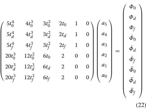
To compute the parameters a0… a5, two main methods

are used in the literature: The Point-to-point method [22] and the Via-point one [23]. The first methodology only requires the expression of the function to be minimized and the values of position, velocity and acceleration of the initial and final time of the movement. The corresponding control algorithm only needs to run once. For each joint, the following relation is used [22]:

where Φ0,Φ˙0 and Φ¨0 are the position, velocity and accel-eration, respectively, at t0. Φf,Φ˙f and Φ¨f are the position,

velocity and acceleration, respectively, at tf.

The via-point method is recommended to avoid obsta-cles in the space where the robotic system evolves. Not only must the initial and final positions be specified but also a number of desired intermediate positions. This method implies that the algorithm is executed several times. In the case where only one desired intermediate position is specified, the solution is given by [23]:

(17)

Φ(6)=0

(18) Φ(t)=a5t5+a4t4+a3t3+a2t2+a1t+a0

(19)

˙

Φ(t)=5a5t4+4a4t3+3a3t2+2a2t+a1

(20) ¨

Φ(t)=20a5t3+12a4t2+6a3t+2a2

(21)             a5 a4 a3 a2 a1 a0             =             

t05 t 4

0 t

3

0 t

2

0 t0 1

t_f5 t_f4 t_f3 t_f2 tf 1

5_t04 4_t03 3_t02 2_t0 1 0

5_t4 f 4t

3

f 3t

2

f 2tf 1 0

2_Ot03 12_t02 6._t0 2 0 0

20t_f3 12t2

where td is an intermediate instant satisfying t0<td<tf. Φd,Φ˙dandΦ¨d are the position, velocity and acceleration, respectively, at td.

The control law

Let impose to the bipedal robotic described by (1) to fol-low the folfol-lowing stable second order linear input–out-put behavior:

where KP,1∈Rn×n and Kv,1∈Rn×n are two positive

defi-nite diagonal matrices chosen to guarantee global stabil-ity, desired performances and decoupling proprieties for the controlled system. For a desired bandwidth λ and a critically damped closed-loop performance, we must select:

As the dynamic modeling of the bipedal robot is known, Kp,1andKv,1 are computed offline to satisfy global

stability conditions.

Using (1) and (23), the control law of the bipedal robot during the SSP is deduced as:

The jerk optimal algorithm

In this section, we propose a new algorithm for the jerk optimal control different from those of the point-to-point and via-Point conventional approaches. The differ-ent steps composing the proposed algorithm for the case study of the bipedal robot for which the swing foot must follow the semi elliptic trajectory are described below:

(22)             

5_t04 4_t03 3_t02 2_t0 1 0

5t4

d 4t

3

d 3t

2

d 2td 1 0

5_t4

f 4t

3

f 3t

2

f 2tf 1 0

20_t3

0 12t

2

0 6t0 2 0 0

20_t3 d 12t

2

d 6td 2 0 0

20_t3 f 12t

2

f 6tf 2 0 0

                           a5 a4 a3 a2 a1 a0               =                        Φ0 Φd Φf ˙ Φ0 ˙ Φd ˙ Φ_f ¨ Φ0 ¨ Φ_d ¨ Φf                        (23) _¨

Φ− ¨Φd+Kv,1Φ˙− ˙Φd+KP,1(Φ−Φd)=0

(24)

Kp,1=diag

2

(25)

Kv,1=diag[2]

(26) U=D−1M(Φ)Φ¨_d−Kv,1Φ˙− ˙Φ_d−KP,1(Φ−Φ_d)

+D−1H

Φ,Φ˙+D−1G(Φ)

i. For desired initial and final Cartesian positions of the toe of the swing foot, compute the initial joint posi-tion vector фin and the final joint position vector фf using the inverse kinematic model (5).

ii. Generate the polynomial trajectories φa, φ˙a and

¨

φa described by (18–20) using the Point-to-Point

method according to the relation (11).

iii. Generate the semi-ellipsoidal Cartesian trajectories, according to relations (9–11).

iv. Generate the desired joint trajectories φd, φ˙d and φ¨d

using (4–6).

v. Compute the jerk optimal control law U(t) using (26). vi. Implement the control law U(t) for the free robotic

system described by the dynamical model (1).

vii. Generate the Cartesian trajectories Xt) and _X˙_{(t) by}

applying the direct kinematic model (2) and the dif-ferential kinematic model (3). ф(t) and _φ˙_{(t) are}

sup-posed to be measured via online sensors.

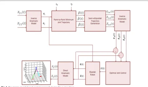
Steps iii to vii must be applied at every time iteration. Figure 1 explains necessary steps for the achievement of the jerk control approach.

The differences between the proposed approach and the conventional ones can be summarised as follows: first, the reference trajectory of the swing foot is planned in the Cartesian space with constraints on positions, velocities and accelerations at every time iteration whereas for the point-to-point method constraints are to be found only at the boundary conditions and for the via-point method these constraints must also include intermediary posi-tions, their velocities and their accelerations. Moreover, the proposed approach uses a trigonometric expression of desired trajectories that depends on a fifth order polyno-mial instead of just having recourse to a fifth order poly-nomial as done for the conventional approaches.

The proposed method of optimal jerk control is designed in order to reduce significantly the time of implementation. As trajectories are planned in the Car-tesian space system whereas control laws are expressed in the joint space, it does combine benefits of trigono-metric and polynomial functions. Indeed, trigonotrigono-metric functions require fewer resources for real time imple-mentation whereas polynomial functions give smoother dynamics and fewer vibrations.

Active stiffness controller

give a solution for such force/position control problem and ensure a stable motion of the bipedal robot. Using an impedance controller to generate a walking cycle, as pro-posed in [24], imposes for the implementation of the con-trol law the availability of force, acceleration and gravity sensors. However, it is well known that this type of sen-sors can cause many problems related to precision and sensibility to noise measurements. To overcome these locks, we propose in this section an alternative solu-tion: A stiffness controller without gravity compensation requiring only position and velocity sensors. To ensure an elastic and robust contact with the ground by elimi-nating the gravity term from the control law, we impose the following virtual model for the contact force:

where Kd∈R3×3 is the stiffness matrix and JT+ is the

pseudo-inverse of the transpose Jacobian matrix of the bipedal robotic system at the contact point. Expressing F

in the joint space, we get:

(27) F =Kd(Xd−X)+

JT+G(Φ)

(28)

F =KdJ(Φd−Φ)+

JT+G(Φ)

Let impose, now, to the constrained bipedal robotic model (8) to follow the following stable second order lin-ear input–output behaviour:

where Kp,2∈Rn×n and Kv,2∈Rn×n are two positive defi-nite diagonal matrices chosen to guarantee global stabil-ity, desired performances and decoupling proprieties for the controlled constrained system (8). Using (28) in (8), we get:

The control law of the bipedal robot during the con-strained phases is deduced as:

The control law (31) is then designed such that the common gravity compensation term found in many research works in the literature is eliminated thanks to the contact force virtual model proposed in (28). This fur-ther gives more robustness to the control law. The control law (31) has also the advantage to reduce the number of

(29)

_¨

Φ− ¨Φ_d

+Kv,2_˙

Φ− ˙Φ_d

+KP,2(Φ−Φ_d)=0

(30)

M(Φ)Φ¨ +H

Φ,Φ˙

=DU−JTKdJ(Φ−Φd)

(31) U =D−1(JTK_dJ−M(Φ)Kp,2)(Φ−Φ_d)

−D−1M(Φ)Kv,2.Φ˙ +D− 1

sensors. To be implemented, it is clear that only position and velocity sensors are needed.

Finally, to achieve a walking cycle and produce alter-nate footsteps, the minimum jerk controller (26) and the active stiffness controller (31) are combined to switch successively between the SSP described by the robotic model (1), and the IP and DSP described by the con-strained robotic model (8).

Simulation results

Simulation results are carried out using the three dimen-sional model of a 12 DOF bipedal robot described by the robotic dynamical models established in [25], the kin-ematic model described in [26] for the physical param-eters given in Table 1. The initial and the final Cartesian positions are chosen, respectively, as follows:

The initial posture of the bipedal robot is shown in the 3D space by Fig. 2. The bipedal robot evolves in rough terrain characterized by the nonlinear stiffness parameter described by:

where kd =  2000. Furthermore, we consider a

Gauss-ian noise of 0.01° mean and 0.01° standard deviation for the joint position measurements and 0.02° s−1 _{mean and}

0.02° s−1 _{standard deviation for the joint velocity}

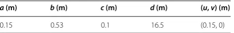
meas-urements. To generate a semi-elliptical trajectory in the sagittal plane similar to a walking step of 0.5 s duration, parameters involved in the 3D Cartesian desired trajec-tory (9) take the values given in Table 2.

Xin= [0 0.53 0]T, Xd =[0.35 0.53 0]T

Kd =[1+500 sin(t)]diag [kd kd kd] _{stability conditions of the desired dynamics (}Position and velocity gain matrices related to the global _{23) and (29)}

are, respectively satisfied by choosing:

where I12 is the identity matrix of twelve order.

Due to very small changes of the Cartesian compo-nent along the y-axis, only the evolution of variables in

Kp,1=625I12, Kv,1=50I12

Kp,2=104I12, Kv,2=200I12

Table 1 Physical parameters of the robot

Link ki (m) li (m) mi (Kg) Inertia about center of mass (Kg m−2₎

iix iix iix

Right foot 0.034 0.034 1.015 0.001 0.001 0.001

Right leg 0.184 0.241 3.255 0.051 0.051 0.051

Right thigh 0.184 0.240 7.000 0.113 0.113 0.113

Pelvis 0.021 0.178 9.940 0.112 0.112 0.112

Left thigh 0.240 0.184 7.000 0.113 0.113 0.113

Left leg 0.241 0.184 3.255 0.051 0.051 0.051

Left foot 0.034 0.034 1.015 0.001 0.001 0.001

-0.2 _{-0.1 0}

0.1 _{0.2 0.3}

0.4 _0.5 -0.4 -0.20

0.20.4 0.60.8

0 0.2 0.4 0.6 0.8 1 1.2

Y X

Z

Fig. 2 Initial posture of the bipedal robot in the 3D space

Table 2 Parameters of the cartesian desired trajectory

a (m) b (m) c (m) d (m) (u, v) (m)

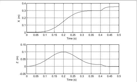
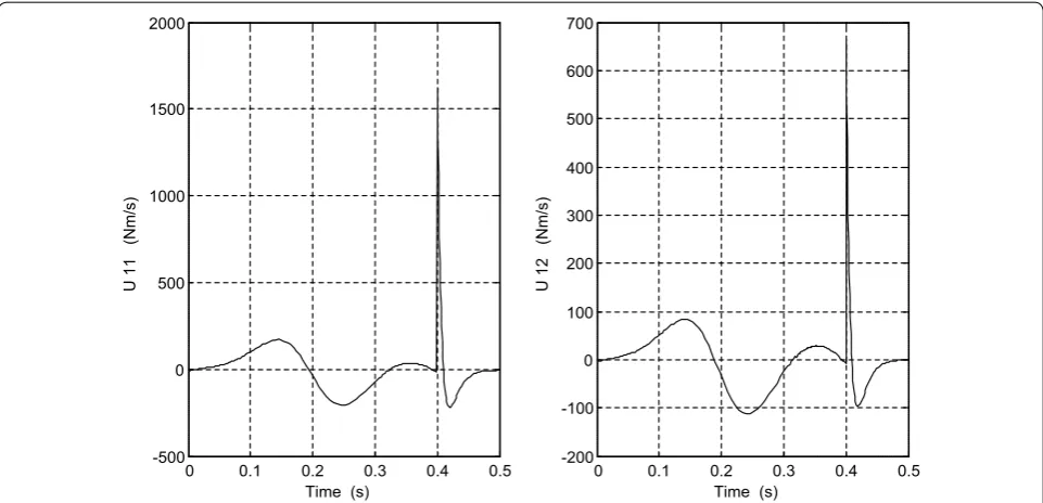
the x and z axis are presented. The Cartesian components along x and z axis of the swing foot during a walking step are emphasized by Fig. 3 whereas Fig. 4 shows the evolu-tion of the ground reacevolu-tion force. Figure 5 shows involved control laws during the same walking step where U11 and U12 are defined as the output of ankle joints. Finally, Fig. 6 presents a gait pattern generation composed by three steps.

Simulation results emphasize the efficiency of the control laws as perturbations and rough terrain have no effect on the bipedal robot trajectory. Compared to previous work found in [24], not only fewer sensors are needed in the implementation of the control laws but the semi-elliptical trajectory duration has been also improved to 0.5 s. It corresponds to an enhanced

0 0.05 0.1 0.15 0.2 0.25 0.3 0.35 0.4 0.45 0.5 0

0.1 0.2 0.3 0.4

Time (s)

X (m)

0 0.05 0.1 0.15 0.2 0.25 0.3 0.35 0.4 0.45 0.5 -0.05

0 0.05 0.1 0.15

Time (s)

Z (m)

Fig. 3 Real cartesian components of the swing foot during a walking step

0 0.05 0.1 0.15 0.2 0.25 0.3 0.35 0.4 0.45 0.5 0

20 40 60 80

Time (s)

F

(N

)

velocity of the bipedal robot of 0.75  m  s−1_{. Also, an}

elastic and robust contact with the ground is ensured. This was not guaranteed with the impedance control law.

Conclusion

To produce a path similar to the one generated by a human foot when performing a walking cycle by a bipedal robot, we have proposed, in this paper, a specific walking control

0 0.1 0.2 0.3 0.4 0.5

-500 0 500 1000 1500 2000

Time (s)

U 11 (Nm/s)

0 0.1 0.2 0.3 0.4 0.5

-200 -100 0 100 200 300 400 500 600 700

Time (s)

U 12 (Nm/s)

Fig. 5 Control laws located of the ankle joint of the swing foot during a walking step

-0.2 0 0.2 0.4 0.6 0.8 1

0 0.2 0.4 0.6 0.8 1 1.2

X (m)

Z

(m

)

strategy using an optimal jerk and an active stiffness con-trollers based only on position and velocity sensors. Simulation results performed on a 12 DOF bipedal robot emphasized the efficiency of the control strategy even in presence of sensory noise and rough terrain and prove the superiority of the new algorithm regarding the step dura-tion and the bipedal velocity compared to previous works. Authors’ contributions

AA proposed the jerk optimal controller and carried out simulation results. OB designed the active stiffness controller. Both authors write the final manu-script. Both authors read and approved the final manumanu-script.

Competing interests

The authors declare that they have no competing interests.

Received: 26 November 2015 Accepted: 14 June 2016

References

1. Boubaker O (2013) The inverted pendulum benchmark in nonlinear control theory: a survey. Int J Adv Robot Syst 10:233. http://www. intechopen.com/books/international_journal_of_advanced_robotic_sys- tems/the-inverted-pendulum-benchmark-in-nonlinear-control-theory-a-survey. Accessed May 2016

2. Hasegawa Y, Arakawa T, Fukuda T (2000) Trajectory generation for biped locomotion robot. Mechatronics. 10:67–89. http://www.sciencedirect. com/science/article/pii/S0957415899000525. Accessed May 2016 3. Kim B (2012) Optimal foot trajectory planning of bipedal robots based on

a measure of falling. Int J Adv Robot Syst 9:172. http://www.intechopen. com/journals/international_journal_of_advanced_robotic_systems/ optimal-foot-trajectory-planning-of-bipedal-robots-based-on-a-measure-of-falling. Accessed May 2016

4. Vladareanu L, Tont G, Ion I, Munteanu MS, Mitroi D (2010) Walking robots dynamic control systems on an uneven terrain. Adv Electr Comput Eng 10:145–152. http://www.aece.ro/abstractplus.php?year=2010&number= 2&article=26. Accessed May 2016

5. Aloulou A, Boubaker O. Minimum jerk-based control for a three dimen-sional bipedal robot. In: Jeschke S, Liu H, Schilberg D (eds) Intelligent robotics and applications. Proceedings of the 4th international confer-ence, ICIRA 2011, Aachen, Germany, December 6-8, 2011, Part II. Lecture notes in computer science, vol 7102, Springer, Berlin, Heidelberg, pp 251– 262. http://link.springer.com/chapter/10.1007%2F978-3-642-25489-5_25. Accessed May 2016

6. Hogan N (1984) An organizing principle for a class of voluntary movements J Neurosci 4:2745–2754. http://www.jneurosci.org/con-tent/4/11/2745.short. Accessed May 2016

7. Erkorkmaz K, Altintas Y (2001) High speed CNC system design. Part I: jerk limited trajectory generation and quintic spline interpolation. Int J Mach Tools Manuf 41:1323–1345. http://www.sciencedirect.com/science/arti-cle/pii/S0890695501000025. Accessed May 2016

8. Perumaal SS, Jawahar N (2013) Automated trajectory planner of industrial robot for pick-and-place task. Int J Adv Robotic Syst 10:100. http://www. intechopen.com/books/international_journal_of_advanced_robotic_sys- tems/automated-trajectory-planner-of-industrial-robot-for-pick-and-place-task. Accessed May 2016

9. Gasparetto A, Zanotto V (2008) A technique for time-jerk optimal plan-ning of robot trajectories. Robot Comput Integr Manuf 24:415–426, http://www.sciencedirect.com/science/article/pii/S0736584507000543. Accessed May 2016

10. Mattmüller J, Gisler D (2009) Calculating a near time-optimal jerk-con-strained trajectory along a specified smooth path. Int J Adv Manuf Tech-nol 45:1007–1016. http://www.scopus.com/inward/record.url?eid=2-s2.0-70449523562&partnerID=40&md5=047c0720a43d669d80e74e0bd 91a7c3f. Accessed May 2016

11. Piazzi A, Visioli A (2000) Global minimum-jerk trajectory planning of robot manipulators. IEEE Trans Ind Electron 47:140–149. http://www.scopus. com/inward/record.url?eid=2-s2.0-0034135641&partnerID=40&md5=6 448dd5e3647f33352656b4dfe8668d9. Accessed May 2016

12. Osornio-Rios RA, Romero-Troncoso RJ, Herrera-Ruiz G, Castañeda-Miranda R (2009) FPGA implementation of higher degree polynomial acceleration profiles for peak jerk reduction in servomotors. Robot Comput Integr Manuf 25:379–392. http://www.sciencedirect.com/science/article/pii/ S0736584508000045. Accessed May 2016

13. Simon D, Dan I, Isik (1991) Optimal trigonometric robot joint trajectories. Robotica 9:379–386. http://journals.cambridge.org/action/displayAb stract?fromPage=online&aid=2555076&fileId=S0263574700000552. Accessed May 2016

14. Nguyen KD, Ng TC, Chen IM (2008) On algorithms for planning s-curve motion profiles. Int J Adv Robot Syst 5:99–106. http://www.scopus.com/ inward/record.url?eid=2-s2.0-40549146252&partnerID=40&md5=1f9cfe a647e8d931ebd896db8e829b39. Accessed May 2016

15. Kyriakopoulos KJ, Saridis GN (1988) Minimum jerk path generation. In: Proc. IEEE international conference on robotics and automation, Philadel-phia, PA, USA, 1988, pp 364–369. http://www.scopus.com/inward/record. url?eid=2-s2.0-0023671834&partnerID=40&md5=af5421c5f5cc73fd24ea 4e415a84296d. Accessed May 2016

16. Zeng G, Hemami A (1997) An overview of robot force control. Robotica 15:473–482. http://dx.doi.org/10.1017/S026357479700057X. Accessed May 2016

17. Salisbury JK (1980) Active stiffness control of a manipulator in cartesian coordinates. In: 19th IEEE Conference on decision and control including, the symposium on adaptive processes pp 95–100 http://ieeexplore.ieee. org/stamp/stamp.jsp?tp=&arnumber=4046624&isnumber=4046601. Accessed May 2016

18. Mehdi H and Boubaker O (2011) Position/force control optimized by particle swarm intelligence for constrained robotic manipulators. In: Proc. IEEE International conference on intelligent systems design and applica-tions (ISDA 2011), Cordoba, Spain, pp 190–195. http://ieeexplore.ieee. org/xpl/articleDetails.jsp?arnumber=6121653. Accessed May 2016 19. Mehdi H, Boubaker O (2012) Stiffness and impedance control using

Lya-punov theory for robot-aided rehabilitation. Int J Soc Robot 4:107–119. http://link.springer.com/article/10.1007/s12369-011-0128-5. Accessed May 2016

20. Mehdi H, Boubaker O (2016) PSO-Lyapunov motion/force control of robot arms with model uncertainties. Robotica 34(3):634–651. doi: 10.1017/S0263574714001775. Accessed May 2016

21. Morimoto J, Atkeson GG (2007) Learning Biped Locomotion IEEE Robot Autom Mag 14:41–51 http://ieeexplore.ieee.org/stamp/stamp.jsp?tp=&a rnumber=4264366&isnumber=4263083. Accessed May 2016 22. Miyamoto H, Morimoto J, Doya K, Kawato M (2004) Reinforcement

learn-ing with via-point representation. Neural Netw 17:299–305. http://www. sciencedirect.com/science/article/pii/S089360800300296X. Accessed May 2016

23. Piazzi AA, Visioli A (1997) An interval algorithm for minimum-jerk trajec-tory planning of robot manipulators. In: Proc. 36th IEEE Conference on decision and control, vol 2, pp 1924–1927 http://ieeexplore.ieee.org/ stamp/stamp.jsp?tp=&arnumber=657874&isnumber=14272. Accessed May 2016

24. Aloulou A, Boubaker O A Minimum jerk-impedance controller for plan-ning stable and safe walking patterns of biped robots. Mech Mach Sci 29:385–415. doi:10.1007/978-3-319-14705-5_13. http://link.springer.com/ chapter/10.1007%2F978-3-319-14705-5_13. Accessed May 2016 25. Aloulou A, Boubaker O A Relevant reduction method for dynamic

mod-eling of a seven-linked Humanoid robot in the three-dimensional space. Procedia Eng 41:1277–1284. http://www.sciencedirect.com/science/ article/pii/S187770581202711. Accessed May 2016