R E S E A R C H
Open Access
Sparse signal subspace decomposition
based on adaptive over-complete dictionary
Hong Sun
1,2*, Cheng-wei Sang
1and Didier Le Ruyet
3Abstract
This paper proposes a subspace decomposition method based on an over-complete dictionary in sparse
representation, called “sparse signal subspace decomposition” (or 3SD) method. This method makes use of a novel criterion based on the occurrence frequency of atoms of the dictionary over the data set. This criterion, well adapted to subspace decomposition over a dependent basis set, adequately reflects the intrinsic characteristic of regularity of the signal. The 3SD method combines variance, sparsity, and component frequency criteria into a unified framework. It takes benefits from using an over-complete dictionary which preserves details and from subspace decomposition which rejects strong noise. The 3SD method is very simple with a linear retrieval operation. It does not require any prior knowledge on distributions or parameters. When applied to image denoising, it demonstrates high
performances both at preserving fine details and suppressing strong noise.
Keywords: Subspace decomposition, Sparse representation, Frequency of components, PCA, K-SVD, Image denoising
1 Introduction
Signal subspace methods (SSMs) are efficient techniques to reduce the dimensionality of data and to filter out noise [1]. The fundamental idea under SSM is to project the data on a basis made of two subspaces, one mostly contain-ing the signal and the other the noise. The two subspaces are separated by a thresholding criterion associated with some measures of information.
The two most popular methods of signal subspace decomposition are wavelet shrinkage [2] and principal component analysis (PCA) [3]. Both techniques have proved to be quite efficient. However, wavelet decompo-sition depending on signal statistics is not equally adapted to different data and requires some knowledge on prior distributions or parameters of signals to efficiently choose the thresholds for shrinkage. A significant advantage of the PCA is its adaptability to data. The separation crite-rion is based on energy which may be seen as a limitation in some cases as illustrated in the next section.
*Correspondence: [email protected]
1School of Electronic Information, Wuhan University, Luojia Hill, Wuhan
430072, China
2Signal and Image Processing Department, Telecom ParisTech, 46 rue Barrault,
75013 Paris, France
Full list of author information is available at the end of the article
In recent years, sparse coding has attracted significant interest in the field of signal denoising [4]. A sparse rep-resentation is a decomposition of a signal on a very small set of components of an over-complete basis (called dic-tionary) which is adapted to the processed data. A difficult aspect for signal subspace decomposition based on such a sparse representation is to define the most appropri-ate criterion to identify the principal components (called atoms) from the learned dictionary to build the principal subspace. The non-orthogonal property of the dictionary does not allow to use the energy criterion for this purpose, as done with PCA.
To solve this problem, we introduce a new criterion to measure the importance of atoms and propose a SSM under the criterion of the occurrence frequency of atoms. We thus make benefit both from the richness of over-complete dictionaries which preserves details of infor-mation and from signal subspace decomposition which rejects strong noise.
The remainder of this paper is organized as follows: Section 2 presents two related works to signal decomposi-tion. Section 3 introduces the proposed sparse signal sub-space decomposition based on the adaptive over-complete dictionary. Some experimental results and analysis are presented in Section 4. Finally, we draw the conclusion in Section 5.
2 Review of PCA and sparse coding methods We start with a brief description of two well-established approaches to signal decomposition that are relevant and related to the approach proposed in the next section.
2.1 PCA-based subspace decomposition
The basic tool of SSM is principal component analysis (PCA). PCA makes use of an orthonormal basis to cap-ture on a small set of vectors (the signal subspace) as much energy as possible from the observed data. The other basis vectors are expected to contain noise only, and the signal projection on these vectors is rejected.
Consider a data set xm∈RN×1 M
m=1 grouped in a
matrix formXof sizeN ×M: X = {xm}Mm=1. The PCA
is based on singular value decomposition (SVD) with singular valuesσiin descending order obtained from:
X=UA=UVT (1) whereUandVare unitary matrices of sizesN×Nand M×M, respectivelyUTU=IN,VTV=IM, and =
diag [σ1,· · ·,σr] ,0
0
of sizeN×Mwithσ1≥σ2≥ · · · ≥
σr > 0,{σi}ri=1 are positive real known as the singular
values ofXwith rankr(r≤N).
Equation (1) can be rewritten in a vector form as:
[x1 x2· · ·xm· · ·xM]
=[u1 u2· · ·un· · ·uN] . [α1 α2· · ·αm· · ·αM] (2)
whereU= un∈RN×1 N
n=1andA=
αm∈RN×1 M
m=1.
Equation (2) means that the data set{xm}Mm=1is expressed
on the orthonormal basis{un}Nn=1as{αm}Mm=1.
In the SVD decomposition given in Eq. (1), the standard deviationσiis used as the measurement for identifying the meaningful basis vectorui. PCA takes the firstP(P < r) components{un}Pn=1to span the signal subspace, and the
remainders{un}rn=P+1are considered in a noise subspace
orthogonal to the signal subspace. Therefore, projection on the signal subspace will hopefully filter out noise and reveal hidden structures. The reconstructed signalSˆPCA
of size N × M is obtained by projecting in the signal subspace as:
ˆ
SPCA=[u1· · ·uP 0P+1· · ·0N] . [α1 α2· · ·αm· · ·αM] (3)
The underlying assumption is that information in the data set is almost completely contained in a small lin-ear subspace of the overall space of possible data vectors, whereas additive noise is typically distributed through the larger space isotropically. PCA, using the standard devi-ation as a criterion, implies that the components of the signal of interest in the data set have a maximum variance
and the other components are mainly due to the noise. However, in many practical cases, some components with low variances might actually be important because they carry information relative to the signal details. On the contrary, when dealing with noise with non-Gaussian statistics, it may happen that some noise components may actually have higher variances. At last, note that it is often difficult to provide a physical meaning to the orthonormal basis{ui}ri=1of the SVD decomposition (Eq. (2)) although
they have a very clear definition in the mathematical sense as orthogonal, independent, and normal. It is there-fore difficult to impose known constraints on the signal features when they exist after the principal component decomposition.
2.2 Sparse decomposition
Recent years have shown a growing interest in research on the sparse decomposition of M obser-vations xm∈RN
M
m=1 based on a dictionary
D = {dk}Kk=1 ∈ RN×K. WhenK > N, the dictionary is said to be over-complete.dk ∈ RN is a basis vector, also called an atom since it is not necessarily independent. By learning from data set{xm}Mm=1, the sparse decomposition is the solution of Eq. (4) [4]:
{D,αm} =argmin D,αm
αm0
+ Dαm−xm22≤ε, 1≤m≤M
(4)
where αm = [αm(1) αm(2) . . . αm(K)]T ∈ RK×1 is the sparse code of the observation xm. The allowed error toleranceεcan be chosen according to the standard devi-ation of the noise. An estimate of the underlying signal {sm}Mm=1 embedded in the observed data set {xm}Mm=1
would be:
ˆ
s1 sˆ2· · · ˆsm· · · ˆsM
=[d1 d2· · ·dk· · ·dK] . [α1 α2· · ·αm· · ·αM] or equivalently Sˆ =DA
(5)
where the matrixAof sizeK×Mis composed ofMsparse column vectorsαm.
of the reconstruction, based on the mean-square recon-struction error estimate in the same way as in the PCA method.
On the other hand, we note that the dictionary D, a basis in sparse decomposition, is produced by learning noisy data set{xm}Mm=1, so the basis vectors{dk}Kk=1should be decomposed into a principal subspace and a residual subspace. However, it is impossible to exploit an energy-constrained subspace since {dk}Kk=1 are not necessarily orthogonal or independent.
3 The proposed sparse subspace decomposition In this section, we introduce a novel criterion to the subspace decomposition over a learned dictionary and a corresponding index of significance of the atoms. Then we propose a signal sparse subspace decomposition (3SD) method under this new criterion.
3.1 Weight vectors of learned atoms
At first, we intend to find out the weight of the atoms. In the sparse representation given in (5), coefficient matrix
Ais composed byMsparse column vectorsαm, eachαm representing the weight of the observation xm, a local parameter for them-th observation. Let us consider the row vectors{βk}Kk=1of coefficient matrixA:
A=[α1α2 · · · αM]
= ⎡ ⎢ ⎢ ⎢ ⎣
α1(1) α2(1) · · · αM(1)
α1(2) α2(2) · · · αM(2) ..
. ... . .. ...
α1(K) α2(K) · · · αM(K) ⎤ ⎥ ⎥ ⎥ ⎦= ⎡ ⎢ ⎢ ⎢ ⎣ β1 β2 .. . βK ⎤ ⎥ ⎥ ⎥ ⎦
where βk=[α1(k) α2(k) . . . αM(k)]∈R1×M (6)
Note that the row vectorβk is not necessarily sparse. Then Eq. (5) can be rewritten as:
ˆ
S=DA
=[d1· · ·dk· · ·dK] .
βT1 · · ·βTk · · ·βTK
T (7)
Equation (7) means that the row vectorβkis the weight of the atomdk, which is a global parameter over the data set X. Denoting βk0the 0 zero pseudo-norm of βk. βk0is the number of occurrences of atomdk over the data set{xm}Mm=1. We call it the frequency of the atomdk denoted byfk:
fkFrequency(dk|X)= βk0 (8)
In the sparse decomposition, basis vectors{dk}Kk=1are prototypes of signal segments. That allows us to take them
as a signal patterns. Thereupon, some important features of this signal pattern could be considered as a criterion to identify significant atoms. It is demonstrated [5] thatfkis a good description of the signal texture. Intuitively, a signal pattern must occur in meaningful signals with higher fre-quency even with a lower energy. On the contrary, a noise pattern would hardly be reproduced in observed data even with a higher energy.
It is reasonable to take this frequencyfk as a relevance criterion to decompose the over-complete dictionary into a principal signal subspace and a remained noise subspace. Here, we use the word “subspace,” but in fact, these two subspaces are not necessarily independent.
3.2 Subspace decomposition based on over-complete dictionary
Taking vectors {βk}Kk=1, we calculate their 0-norms
{βk0}Kk=1and rank them in descending order as follows.
The indexk of vectors {βk}Kk=1are belonging to the set
C = {1, 2,· · ·,k,· · ·,K}. A one-to-one index mapping functionπis defined as:
π(C→C):k=π(k˜), k,k˜∈C
s.t. βπ(1)0≥βπ(2)0≥ · · · ≥βπ(k˜)0≥ · · · ≥βπ(K)0
(9)
By the permutationπof the row indexkof matrixA=
βT1· · ·βTk · · ·βTK T
, the reordered coefficient matrix A˜
becomes
˜
A=
βTπ(1) βTπ(2)· · ·βTπ(k)· · ·βTπ(K)T (10)
With corresponding reordered dictionaryD˜ = {dπ(k)}Kk=1,
Eq. (7) can be written as:
ˆ
S= ˜DA˜
=dπ(1)· · ·dπ(k)· · ·dπ(K) .
βTπ(1)· · ·βπ(Tk)· · ·βTπ(K) T
(11)
Then, the span of the firstP atoms can be taken as a principal subspaceD(S)P , and the remaining atoms span a noise subspaceD(KN−)Pas:
D(S)P =span{dπ(1),dπ(2),· · ·,dπ(P)}
D(KN−)P=span{dπ(P+1),dπ(P+2),· · ·,dπ(K)}
(12)
ˆ
SP=D(S)P .A(S)P
=dπ(1)· · ·dπ(k)· · ·dπ(P) .
βTπ(1)· · ·βπ(Tk)· · ·βTπ(P) T
(13)
3.3 Threshold of atom’s frequency
Determining the numberPof atoms spanning the signal subspaceD(PS) is always a hard topic especially for wide-band signals. Here,Pis the threshold of atom’s frequency fk to distinguish a signal subspace and a noise subspace. One of the advantages of 3SD is that this thresholdPcan be easily chosen without any prior parameter.
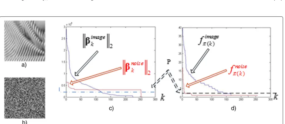
For a noiseless signal even with some weak details, such as the image example in Fig. 1a, the atoms’ frequencies fπ(imagek) s shown in Fig. 1d (in black line) are almost always high except the zero value. For a signal with strong noise, such as the example in Fig. 1b, the atoms’ frequencies fπ(noisek) s shown in Fig. 1d (in red line) are almost always equal to 1 without zero and very few with a value 2 or 3. It is easy to set a thresholdPoffk(dotted line in the Fig. 1d) to separate the signal’s atoms from the noise’s atoms. By contrast, using the values of atom’s energiesβk2s for the
two images shown in Fig. 1c, it is rather a puzzle to identify principal bases.
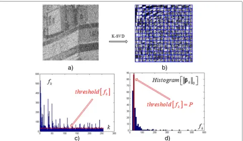
For a noisy signal, such as an image example in Fig. 2a, its adaptive over-complete dictionary (Fig. 2b) consists of atoms of principal signal patterns, strong noise pat-terns, and noisy signal patterns. Principal signal atoms should have higher frequencies, strong noise atoms lower frequencies and noisy signal atoms moderate frequen-cies. Intuitively, the red line (Fig. 2c) should be a suitable thresholdPof the frequenciesfks. In practical implemen-tation, the value ofPcould be simply decided relying on the histogram of fk. As shown in Fig. 2d, one can set
the value offk associated with the maximum point of its histogram toPas follows:
P=arg max Hist k
(βk0) (14)
In fact, the performances in signal analyses by 3SD method are not sensitive to the thresholdP, owed to the dependence of the atoms. To illustrate this point, we take three images, Barbara, Lena, and Boat. Their histograms offkare shown in Fig. 3a with the maximum points in dot-ted lines, 121, 97, and 92, respectively. Figure 3b reports the peak signal-to-noise ratio (PSNR) of the retrieved images SˆP on the signal principal subspace D(PS) with respect to P. We can see that the PSNRs of the results remain the same in a large range around the maximum points (in dotted lines). Consequently, taking the value of fkassociated to the maximum point of its histogram as the thresholdPis a reasonable solution.
4 Results and discussion
4.1 Signal decomposition methods
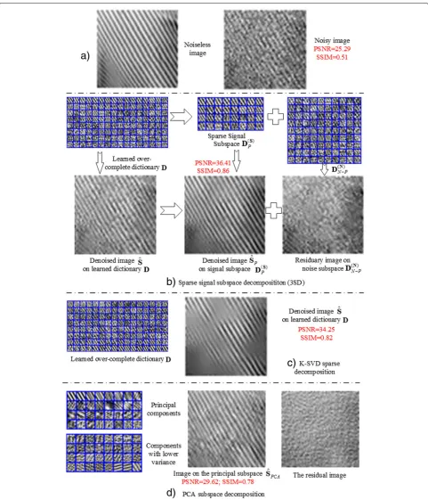
Taking a part of the noisy Barbara image (Fig. 4a), we show an example of the sparse signal subspace decomposition (3SD) and the corresponding retrieved image (Fig. 4b). For comparison, the traditional sparse decomposition and the PCA-based subspace decomposition are shown in Fig. 4c, d. We use the PSNR to assess the noise removal perfor-mance:
PSNR=20·log10MAX{S(i,j)} −10·log10[MSE]
MSE= 1
IJ
I−1
i=0
J−1
j=0
S(i,j)− ˆS(i,j)
2
(15)
Fig. 2The thresholdPof the frequenciesfks.aNoisy image.bOver-complete dictionaryD.cFrequency ofdk.dHistogram ofdk’s frequency
and the structural similarity index metric (SSIM) between the denoised image and the pure one to evaluate the preserving detail performance:
SSIM(S,Sˆ)= (2uSuSˆ+c1)(2σSSˆ+c2)
u2S+u2ˆ
S+c1 σ 2
S+σSˆ2+c2
(16)
whereuxis the average ofx,σx2is the variance ofx,σxyis the covariance ofxandy, andc1andc2are small variables
to stabilize the division with a weak denominator.
Let us look at the proposed sparse signal subspace decomposition on the top of Fig. 4b. The 128 atomsdks of the learned over-complete dictionaryD are shown in descending order of their energies measured by βk2.
The 32 principal signal atoms are chosen from the dic-tionaryDunder the frequency criterion. They are shown in descending order of their frequencies measured by βk0 composing a signal subspace D(S)32. We can see
that some of the principal atoms are not among the first 32 atoms with the largest energy in the over-complete
Fig. 4Signal decompositions.aImage sample.bSparse Subspace decomposition.cSparse decomposition.dSubspace decomposition
dictionaryD. The retrieved images are shown at the bot-tom of Fig. 4b. The imageSonDis apparently denoised. The image Sˆ on the signal subspace D(32S) improves
subspaceD(96N)contains some very noisy information. This is because the atoms of the over-complete dictionary are not independent.
For the same example, the classical sparse decompo-sition is shown in Fig. 4c, using the K-SVD algorithm [6] in which the allowed error tolerance ε (in Eq. (4)) is set to a larger value to filter out noise. The retrieved image S has a high PSNR = 29.62, but it has obvi-ously lost the weak information with SSIM = 0.82. This is because signal distortion and residual noise can-not be minimized simultaneously at dictionary learning by Eq. (4).
In another comparison, the PCA-based subspace decomposition is shown in Fig. 4d. The 64 components are orthonormal and the 32 principal components are of the largest variance. The retrieved image by projecting on the signal subspace is rather noisy with PSNR = 29.62. This is because it cannot suppress strong noise and pre-serve weak details of information only using the variance criterion.
4.2 Application to image denoising
The application of 3SD to image denoising is presented here. A major difficulty of denoising is to separate the underlying signal from the noise. The proposed 3SD method could win this challenge. In the 3SD method, the important components are selected from the over-complete dictionary relying on their occurrence number over the noisy image set. Evidently, the occurrence num-bers would be large for the signal, even for weak details, such as edges or textures. On the other hand, the occur-rence numbers would be low for different kinds of white Gaussian or non-Gaussian noises, even strong at intensity. The 3SD algorithm for image denoising is presented as follows:
Input: Noisy imageX Output: Denoised imageSˆ
- Sparse representation{D,A}: using K-SVD algorithm [6] by (4)
- Identify principal atoms fromDbased onA:
Compute the frequencies of atoms {βk0}Kk=1according to (6) and (8) Get the permutationπsorting the index
kof{βk0}Kk=1by (9)
Compute the thresholdPby (14) - Obtain the signal principal atoms{dπ(k)}Pk=1
by (12)
- Reconstruct imageSˆPby (13)
In this application, we intend to preserve faint signal details under a situation of strong noise.
In the experiments, dictionaries usedDs of size 64×256 (K=256 atoms), designed to handle image patchesxmof sizeN=64=8×8 pixels.
4.3 Image denoising
A noisy Lena imageX=S+Vwith an additive zero-mean white Gaussian noiseVis used. The standard deviation of noise isσ = 35. A comparison is made between the 3SD method and the K-SVD method [6] which is one of the best denoising methods reported in the recent literatures. From the results shown in Fig. 5, the 3SD method out-performs the K-SVD method by about 1 dB in PSNR and by about 1% in SSIM (depending on how much details in the images and how faint the details). In terms of subjec-tive visual quality, we can see that the corner of the mouth and the nasolabial fold with weak intensities are much better recovered by the 3SD method.
4.4 SAR image despeckling
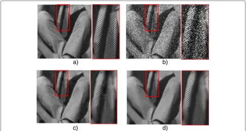
In the second experiment, a simulated SAR image with speckle noise is used. Speckle is often modeled as mul-tiplicative noise as x(i,j) = s(i,j)v(i,j) where x, s, and vcorrespond to the contaminated intensity, the original intensity, and the noise level, respectively.
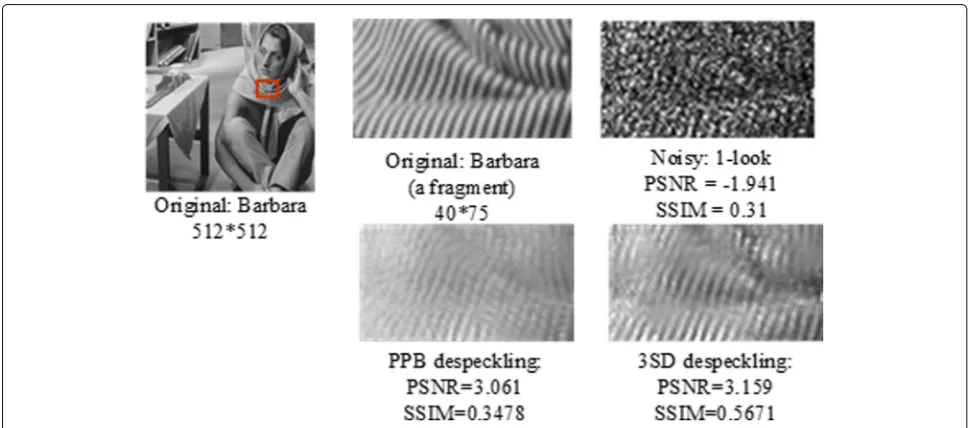
Figure 6 shows the despeckling results of a simulated one-look SAR scenario with a fragment of the Barbara image. A comparison is made with 3SD method and a probabilistic patch-based (PPB) filter based on nonlocal means approach [7] which can cope with non-Gaussian noise. We can see that PPB can well remove speckle noise. However, it also removes the low-intensity details. The 3SD method shows advantages at preserving fine details and at suppressing strong noise.
4.5 Comparison with BM3D method
With a spatial complicated image scene, we make a com-parison of the 3SD-based denoising method with the BM3D algorithm [8], one of the best methods especially for image denoising reported in many recent literatures.
The effectiveness of any signal analysis method depends on the different conditions in different applications. For the image denoising application, the signals involved should be homogeneous. Therefore, a procedure of group-ing is generally adopted to select homogeneous pixels. In the BM3D method, a block-matching grouping is taken before filtering. We adopt the same grouping technique and then filter each homogeneous group by the proposed 3SD method.
Firstly, we take a 256×256 Barbara image (Fig. 7a) with a strong additive zero-mean white Gaussian noise where
σ = 70 (Fig. 7b). The denoising result by the BM3D algorithm is shown in Fig. 7c. It displays a quite high per-formance. The denoising result by the 3SD-based method is shown in Fig. 7d. It demonstrates a higher PSNR and a higher SSIM and a better subjective visual quality over the BM3D algorithm.
Fig. 5Image denoising comparing the proposed 3SD method with the K-SVD method
−0.1042. Figure 8b shows the despeckling result by the PPB method [7], in which grouping is realized based on nonlocal similarity and filtering is implemented by aver-aging each homogeneous group. The despeckled image is too smooth due to average filtering. Figure 8c shows the despeckling result by the BM3D-based method [9], in which grouping is realized based on similar 2-D frag-ments and filtering is implemented by Wiener shrinkage
coefficients from the energy of the 3-D transform coeffi-cients. The despeckled image is much better in PSNR and in SSIM, but it seems a little noisy still due to the used energy criterion which is not effective enough to sepa-rate noise elements from the principal elements. Figure 8d shows the despeckling result by the proposed 3SD-based method, in which grouping is realized based on non-local similarity [7] and filtering is implemented by the
Fig. 7Denoising for spatial complicated image scene comparing BM3D method with 3SD-based method.aOriginal: Barbara (a fragment) 256∗256.
bNoisy:σ=70; PSNR=11.22; SSIM=0.142.cBM3D denoising: PSNR=24.08; SSIM=0.7026.d3SD denoising: PSNR=24.21; SSIM=0.765
proposed sparse subspace decomposition. The despeckled image demonstrates some advantages of the 3SD method at preserving fine details and at suppressing speckle noise, attributed to the principal subspace decomposition.
5 Conclusions
We proposed a method of sparse signal subspace decom-position (3SD). The central idea of the proposed 3SD is to identify principal atoms from an adaptive over-complete dictionary relying on the occurrence frequency of atoms over the data set (Eq. (8)). The atom frequency is measured by zero pseudo-norms of weight vectors of atoms (Eqs. (6) and (8)). The principal subspace is spanned by the maximum frequency atoms (Eq. (12)).
The 3SD method combines the variance criterion, the sparsity criterion, and the component’s frequency crite-rion into a uniform framework. As a result, it can iden-tify more effectively the principal atoms with the three important signal features. On the contrary, PCA uses only variance criterion and sparse coding method uses the variance and the sparsity criterions. In those ways, it is more difficult to distinguish weak information from strong noise.
Another interesting asset of the 3SD method is that it takes benefits from using an over-complete dictionary which reserves details of information and from subspace decomposition which rejects strong noise. On the con-trary, some undercomplete dictionary methods [10] and
some sparse shrinkage methods [11, 12] might lose weak information when suppressing noise.
Moreover, the 3SD method is very simple with a lin-ear retrieval operation (Eq. (13)). It does not require any prior knowledge on distribution or parameter to deter-mine a threshold (Eq. (14)). On the contrary, some sparse shrinkage methods, such as [11], necessitate non-linear processing with some prior distributions of signals.
The proposed 3SD could be interpreted as a PCA in sparse decomposition, so it admits straightforward exten-sion to applications of feature extraction, inverse prob-lems, or machine learning.
Acknowledgements
The idea of the sparse signal subspace decomposition here arises through a lot of deep discussions with Professor Henri Maitre at Telecom ParisTech in France; he also gave suggestion on the structure of the manuscript.
Funding
This work was supported by the National Natural Science Foundation of China (Grant No. 60872131).
Authors’ contributions
HS proposed the idea, designed the algorithms and experiments, and drafted the manuscript. CWS gave suggestion on the design of the algorithm, realized the algorithms, and carried out the experiments. DLR gave suggestions on the mathematical expressions of the manuscript and experiment analysis as well as explanation and helped draft the manuscript. All authors read and approved the final manuscript.
Competing interests
The authors declare that they have no competing interests.
Publisher’s Note
Springer Nature remains neutral with regard to jurisdictional claims in published maps and institutional affiliations.
Author details
1School of Electronic Information, Wuhan University, Luojia Hill, Wuhan
430072, China.2Signal and Image Processing Department, Telecom ParisTech,
46 rue Barrault, 75013 Paris, France.3CEDRIC Laboratory, CNAM, 292 rue Saint
Martin, 75003 Paris, France.
Received: 13 September 2016 Accepted: 17 July 2017
References
1. K Hermus, P Wambacq, HV Hamme, A review of signal subspace speech enhancement and its application to noise robust speech recognition. EURASIP J. Adv. Signal Process. 888–896 (2007). doi:10.1155/2007/45821 2. DL Donoho, IM Johnstone, G Kerkyacharian, D Picard, Wavelet shrinkage: asymptopia? J. R. Stat. Soc. Ser. B.57, 301–369 (1995). http://citeseer.ist. psu.edu/viewdoc/summary?doi=10.1.1.162.1643
3. DW Tufts, R Kumaresan, I Kirsteins, Data adaptive signal estimation by singular value decomposition of a data matrix. IEEE Proc.70(6), 684–685 (1982). doi:10.1109/PROC.1982.12367
4. M Elad, M Aharon, Image denoising via sparse and redundant representations over learned dictionaries. IEEE Trans. Image Process.
15(12), 3736–3745 (2006). doi:10.1109/TIP.2006.881969
5. G Tartavel, Y Gousseau, G Peyré, Variational texture synthesis with sparsity and spectrum constraints. J. Math. Imaging Vis.52(1), 124–144 (2015). doi:10.1007/s10851-014-0547-7
6. M Aharon, M Elad, A Bruckstein, K-SVD: an algorithm for designing overcomplete dictionaries for sparse representation. IEEE Trans. Signal Process.54(11), 4311–4322 (2006). doi:10.1109/TSP.2006.881199 7. CA Deledalle, L Denis, F Tupin, Iterative weighted maximum likelihood
denoising with probabilistic patch-based weights. IEEE Trans. Image Process.18(12), 2661–2672 (2009). doi:10.1109/TIP.2009.2029593
8. K Dabov, A Foi, V Katkovnik, K Egiazarian, Image denoising by sparse 3-D transform-domain collaborative filtering. IEEE Trans. Image Process.16, 2080–2095 (2007). doi:10.1109/TIP.2007.901238
9. S Parrilli, M Poderico, CV Angelino, L Verdoliva, A nonlocal SAR image denoising algorithm based on LLMMSE wavelet shrinkage. IEEE Trans. Geosci. Remote Sens.50, 606–616 (2012). doi:10.1109/TGRS.2011.2161586 10. F Porikli, R Sundaresan, K Suwa, SAR depeckling by sparse reconstruction
on affinity nets. EUSAR2012.18, 796–799 (2012). https://www.research gate.net/publication/232905473_SAR_Despeckling_by_Sparse_ Reconstruction_on_Affinity_Nets_SRAN
11. A Hyvarinen, P Hoyer, E Oja, Sparse code shrinkage for image denoising. IEEE World Congr. Comput. Intell.2, 59–864 (1998). doi:10.1109/IJCNN. 1998.685880
12. R Malutan, R Terebes, C Germain, Speckle noise removal in ultrasound images using sparse code shrinkage. 5th IEEE Conf. E-Health Bioeng. Conf.