https://doi.org/10.5194/jsss-7-91-2018
© Author(s) 2018. This work is distributed under the Creative Commons Attribution 4.0 License.
Combined distributed Raman and Bragg fiber
temperature sensing using incoherent optical frequency
domain reflectometry
Max Koeppel1,5, Stefan Werzinger1, Thomas Ringel1,2, Peter Bechtold2, Torsten Thiel3, Rainer Engelbrecht4, Thomas Bosselmann2, and Bernhard Schmauss1,5
1Institute of Microwaves and Photonics, Friedrich-Alexander University Erlangen-Nürnberg (FAU), Cauerstr. 9, 91058 Erlangen, Germany
2Siemens AG, Corporate Technology, Guenther-Scharowsky-Str. 1, 91050 Erlangen, Germany 3Advanced Optics Solutions GmbH (AOS), Overbeckstr 39a, 01139 Dresden, Germany 4Polymer Optical Fiber Application Center, Technische Hochschule Nürnberg Georg Simon Ohm,
90489 Nuremberg, Germany
5SAOT Erlangen Graduate School In Advanced Optical Technologies, Friedrich-Alexander University Erlangen-Nürnberg (FAU), Paul-Gordan-Str. 6, 91052 Erlangen, Germany
Correspondence:Max Koeppel (max.koeppel@fau.de)
Received: 29 September 2017 – Revised: 18 December 2017 – Accepted: 2 January 2018 – Published: 21 February 2018
Abstract. Optical temperature sensors offer unique features which make them indispensable for key indus-tries such as the energy sector. However, commercially available systems are usually designed to perform either distributed or distinct hot spot temperature measurements since they are restricted to one measurement prin-ciple. We have combined two concepts, fiber Bragg grating (FBG) temperature sensors and Raman-based dis-tributed temperature sensing (DTS), to overcome these limitations. Using a technique called incoherent optical frequency domain reflectometry (IOFDR), it is possible to cascade several FBGs with the same Bragg wave-length in one fiber and simultaneously perform truly distributed Raman temperature measurements. In our lab we have achieved a standard deviation of 2.5 K or better at a spatial resolution in the order of 1 m with the Raman DTS. We have also carried out a field test in a high-voltage environment with strong magnetic fields where we performed simultaneous Raman and FBG temperature measurements using a single sensor fiber only.
1 Fiber optical temperature sensing
An important application for fiber sensors is temperature monitoring. One of the main advantages of fiber optic tem-perature sensors is that long distances can be covered and that the sensor fibers are insensitive to electromagnetic fields. This allows fiber optic sensors to be employed in all kinds of industrial environments and energy facilities (Hu et al., 2011). Several sensors can be cascaded or multiplexed to measure at a series of distant locations using only a single, centrally installed measurement unit, which reduces costs and complexity.
There are various different measurement concepts that are either based on temperature-dependent scattering
phenom-ena (Rayleigh, Brillouin, Raman scattering; Ukil et al., 2012) or employ distinct temperature sensitive fiber components such as fiber Bragg gratings (FBGs; Kersey et al., 1997).
While scattering-based concepts enable truly distributed temperature sensing (DTS), FBG sensors are better suited for the monitoring of hot spots at distinct positions with a good temperature resolution.
Zaidi et al. (2012) combined Raman DTS and FBGs for dynamic strain sensing. However, they used two separate fibers (single-mode for FBGs, multimode for Raman DTS) and a time domain interrogation approach which was not suitable to measure the absolute Bragg wavelength.
in-coherent optical frequency domain reflectometry (IOFDR), which is implemented with a tunable laser source (TLS) for interrogation and uses only one single-mode fiber (Köppel et al., 2017).
2 Incoherent optical frequency domain reflectometry
2.1 Spatially resolved backscatter and reflection measurements with incoherent optical frequency domain reflectometry
For both concepts, Raman DTS and FBG temperature sens-ing, a method to spatially resolve the backscattered and re-flected light along the fiber is needed. In a Raman DTS sys-tem, the temperature measurement is based on the power ra-tio of the Raman Stokes and anti-Stokes backscattering com-ponents, whereas for the FBG sensors the spatial resolution, in addition to the wavelength resolution, is crucial to separate the individual FBG sensors.
Conventional optical time domain reflectometry (OTDR) systems launch an optical pulse into the fiber and measure the backscattered and reflected light over time. This so-called impulse responsehF(t) can be related to spatial fiber coordi-nates via the group velocity of light in the fiber resulting in a backscattering/reflection profileR(z).
However, the same information can be obtained by mea-suring the frequency responseHF(f) of the sensor fiber and calculatinghF(t) via the inverse Fourier transform (IFT) as depicted in Fig. 1. This approach is called IOFDR and of-fers various advantages over OTDR, such as a lower peak-to-average power ratio and accurate calibration capabilities. A higher average power leads to a better signal-to-noise ra-tio, whereas calibration techniques allow the full available bandwidth of the components to be used and non-idealities in their frequency response to be compensated.
IOFDR was first used as an alternative to OTDR for fiber fault detection (Ghafoori-Shiraz and Okoshi, 1985). Later, it was also proposed for various fiber sensing applications, including Raman DTS (Karamehmedovic and Glombitza, 2004), distributed strain sensing in polymer optical fibers
ratio in the fiber compared to pulsed operation. However, in order to avoid self-stimulated Brillouin backscattering which would limit the maximum CW optical launch power, it is necessary to spectrally broaden the laser source. We use phase modulation with a noise signal to broaden the laser source to a linewidth of around 6 GHz. This is significantly broader than the Brillouin gain spectrum which has a width in the order of tens of MHz for a standard single-mode fiber. Therefore, Brillouin scattering is effectively suppressed for the fibers and launch powers used in our setup. Moreover, this ensures that the light source operates in the incoherent regime with a sufficiently small coherence length while keep-ing the wavelength accuracy of a narrow-band laser.
In order to measure the frequency responseHF(f) of a sensor fiber, the CW light source is intensity-modulated with frequencies up to about 100 MHz with the stimulus signal of a vector network analyzer (VNA) via a Mach–Zehnder modulator (MZM).
In the sensor fiber, light is backscattered by Rayleigh and Raman scattering or reflected by FBGs. Some of this light is guided in the backward direction in the fiber and even-tually separated using a circulator. An optical filter bank is used to split it up into the different spectral components re-sulting from FBG reflections/Rayleigh and Raman scatter-ing. Each spectral component is detected with a fast photodi-ode. The electrical output signal of the detectors is amplified and fed into the VNA again, which determines the amplitude and phase relative to the electrical stimulus signal that was used to modulate the pump light (see Fig. 2).
Measuring this complex-valued transfer function at many uniformly spaced frequencies and normalizing it to a refer-ence trace gives the discrete frequency response HF(f) of the sensor fiber. Calculating an IFT yields the corresponding impulse responsehF(t) in the time domain. The whole exper-imental measurement system was installed in a portable rack (see Fig. 3), which allows it to be employed flexibly.
Figure 2.Schematic setup of the experimental IOFDR system.
Figure 3.Portable experimental IOFDR system in a rack.
From the reflection/backscatter impulse responsehF(t) the reflection/backscatter profileR(z) is obtained by estimating the DC component and rescaling the abscissa using
z(t)=1
2vgt, (1)
wherevg is the effective group velocity in the sensor fiber. The DC componentHF(f =0) corresponds to an upshift of the reflection/backscatter profile and cannot be measured di-rectly with the VNA. However, it can be accounted for by
subtracting the noise floor offset after the end of the fiber where the mean backscatter level must be zero.
The nominal achievable spatial two-point resolution1z for this approach is given by (Iizuka et al., 1984)
1z= vg
2B, (2)
where B is the electrical measurement bandwidth of the VNA. This value corresponds to the distance between the first zero crossings of the sinc reconstruction kernel if no window is applied and is often presented for comparison. However, even small reflections, e.g., at fiber connectors, cause side lobe artifacts that must be suppressed with the help of an effective window at the cost of a decreased ef-fective spatial resolution.
The maximum unambiguous measurement rangezmaxfor a given bandwidthB is limited by the number of measure-ment frequenciesN, yielding (Iizuka et al., 1984)
zmax= vg
2B ·(N−1)= vg
21f, (3)
with1f resembling the frequency step size of the VNA. For Raman DTS measurements a frequency step size of 30 kHz and a maximum modulation frequency of 99.99 MHz was used. These parameters yield a maximum unambiguous measurement rangezmaxof almost 3.5 km and a nominal spa-tial resolution1zof around 1 m. However, due to the Black-man window of (even) lengthN,
WB(n)=0.42−0.50 cos
2π
N n
+0.08 cos
2π
N 2n
,
n= −N
2, . . .,−1,0,1, . . ., N
2, (4)
3 Fiber Bragg grating temperature sensing
FBGs are point sensors for temperature measurements and therefore suitable for selective thermal hot spot monitoring. Their periodic refractive index modulation causes a narrow-band back reflection at the so-called Bragg wavelength given by the Bragg conditionλB=2neff3, whereneffis the effec-tive refraceffec-tive index of the fiber and 3the grating period. Both of these parameters depend on temperature and strain, resulting in a shift of the Bragg wavelength1λB=λB−λB0 relative to the wavelengthλB0at a reference temperatureT0 and strain. In order to measure temperature changes 1T =
T −T0only, it is necessary that the FBGs are either strain-compensated or mechanically decoupled from any strain.
Generally, the temperature dependence of the Bragg wave-length follows a nonlinear function (Filho et al., 2014), which is usually expanded into a Taylor series:
1λB(T)= ∂λB
∂T 1T + 1 2
∂2λB ∂T21T
2+. . .. (5) In many applications, the linear temperature coefficient ∂λB/∂T is sufficiently accurate. However, for wide tempera-ture ranges and better accuracy, higher order terms should be taken into account in the calibration process.
In our system, the Bragg wavelength of a FBG sensor is determined by examining the reflectivity during a stepped wavelength scan of a tunable laser source (TLS; Werzinger et al., 2016). An array of several FBGs with the same or similar Bragg wavelengths can be separated spatially by performing IOFDR measurements at each wavelength step.
The spectral signatures of the gratings are recon-structed using a model-based compressed sensing approach (Werzinger et al., 2017), where the fixed positions of the FBGs are used as prior knowledge and the reflectivities are estimated directly from the measured frequency response without performing an IFT.
Two FBG arrays, each containing three gratings in a spac-ing of 2 m, were fabricated in a HI1060 FLEX sspac-ingle-mode fiber, which was subsequently recoated. The first grating ar-ray was fabricated without hydrogen loading, reaching re-flectivities of∼0.2 %, whereas for the second grating array
Figure 4.Calibration curves for the FBGs used in the temperature measurement experiment.
a hydrogen-loaded fiber was used, resulting in reflectivities of∼1 %. The low reflectivities were chosen to suppress any crosstalk effects like multiple reflections and spectral shad-owing, which occur if the Bragg wavelengths of the FBGs overlap (Cooper et al., 2001).
Prior to the temperature measurements, a calibration of the Bragg wavelengths over temperature was performed. There-fore, the gratings were installed in a temperature control unit with thermoelectric coolers, and 10 temperature cycles rang-ing from 0 to 80◦C in steps of 10 K were run.
The Bragg wavelengths are determined from the recon-structed reflectivity profiles by a Gaussian fit with a threshold of 20 % (see calibration points in Fig. 4). At a temperature of 20◦C, the grating array with lower reflectivities (labeled FBG 1–3) contains one FBG with a Bragg wavelength of 1540.6 nm and two gratings at 1541.3 nm, whereas all FBGs of the second array (labeled FBG 4–6) are centered around 1538.9 nm. These differences are probably due to the hydro-gen treatment of the second grating array prior to the fabrica-tion and increased fabricafabrica-tion tolerances at low reflectivities. Looking closer at the calibration points in Fig. 4, a slightly nonlinear characteristic can be observed towards lower tem-peratures. Therefore, a second-order polynomial was fitted to the calibration data (see Fig. 4).
The average root mean square error (RMSE) of the calibra-tion curves is approximately 8 pm, which would correspond to a temperature uncertainty of about 0.6 to 0.7 K for these gratings.
4 Distributed Raman temperature sensing
Figure 5.Setup of the filter bank that is used to separate the Raman components and the FBG reflections (the dashed components were added for improved isolation in the field test measurements).
pump wavelengthλ0of 1540 nm. Moreover, a spectral broad-ening occurs due to the interaction between the molecules in a solid medium. The resulting spectra of the two Raman com-ponents can be separated with an optical filter bank. Due to the temperature dependence of the occupation of the energy states in silica, the ratio between the intensity of the anti-Stokes waveIAS,0and the Stokes waveIS,0is also dependent on temperature (Engelbrecht, 2014; Dakin et al., 1985):
IAS,0 IS,0
= f
AS fS
4 ·exp
−h·fvib
kT
. (6)
In Eq. (6), fAS and fS are the frequencies of the anti-Stokes and anti-Stokes wave, respectively,his Planck’s constant andkis Boltzmann’s constant.
For a practical application, Eq. (6) must be extended due to the wavelength dependence of the backscatter capture frac-tionηin a fiber and the differences in the detector sensitivity Rresp. Neglecting the slightly differing fiber attenuation for the Raman components yields
IAS(z) IS(z)
=Rresp,AS
Rresp,S ·ηAS
ηS ·
fAS
fS 4
·exp
−h·fvib
kT
. (7)
5 Calculation of the temperature based on the measured Raman backscattering traces
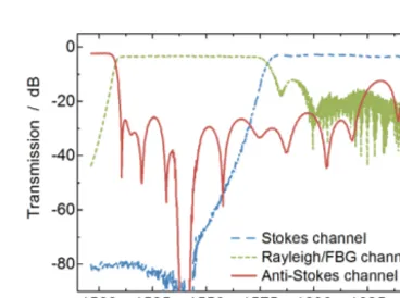
The proposed filter bank setup to separate the Raman Stokes, Raman anti-Stokes backscattering and FBG reflections, de-signed for a pump wavelength of 1540±2 nm, is shown in Fig. 5.
At the input of the filter bank, the Raman anti-Stokes com-ponent, which generally has the lowest power, is split off by a wavelength division multiplexer (WDM). Because of the limited isolation between the WDM outputs, a FBG-based stop filter is necessary in the Raman anti-Stokes channel to block Rayleigh backscatter and the relatively strong FBG reflections in the pump wavelength window. The spectral Rayleigh/FBG content is split off by employing a long-pass edge filter, which is installed after a circulator. The Raman
Figure 6.Measured backscattering spectra at the filter bank outputs (before enhancement) for a 300 m HI1060 FLEX fiber (resolution bandwidth: 1 nm).
Figure 7.Transmission characteristics of the enhanced filter bank setup.
Stokes component can be detected at the output of the long-pass filter.
vari-With our initial setup used for the lab experiment, a very good isolation between the Rayleigh/FBG channel and the two Raman channels of about 70 dB was achieved.
However, due to the large differences in power between the reflections of the FBGs (reflectivities up to approximately
−20 dB) and the Raman backscattering (around−90 dB for a 1 m fiber segment) we have enhanced the isolation between the filter channels by additional FBG-based stop filters in the Raman channels for the field test. The transmission char-acteristics of the enhanced filter bank setup are depicted in Fig. 7.
Furthermore, there is some extent of crosstalk between the channels. Especially the non-ideal separation of the Raman channels must be considered when the temperature is calcu-lated. Moreover, the two filter channels for the Raman com-ponents will generally experience different attenuations,aAS andaS. Therefore, the measured ratio of power in the anti-Stokes and anti-Stokes wave can be expressed as
I0AS(z) I0
S(z) =aAS
aS ·
I AS(z) IS(z)
· 1
1−x + x 1−x
, (8)
wherex is the factor of coupling from the Stokes into the anti-Stokes channel. The various factors can be replaced by two calibration coefficients,C1andC2:
I0AS(z) I0
S(z)
=C1·exp
−h·fvib
kT(z)
+C2. (9)
The coefficientsC1andC2 can be determined from cal-ibration sections where the fiber has a known temperature. For a given temperature T and a fixed (measured) ratio I0AS(z)/I0S(z), Eq. (9) resembles a linear regression prob-lem. To findC1andC2a standard least-squares algorithm is employed.
Eventually, rearranging Eq. (9) gives the temperature pro-fileT(z) along the fiber in dependence of the measured, spa-tially resolved backscatter ratioIAS0(z)/IS0(z) at the outputs of the filter bank:
T(z)= − h·fvib
k·lnI0AS(z)
I0
S(z) −C2
−lnC1
. (10)
Figure 9.Examples of reconstructed FBG reflectivities at three dif-ferent temperatures using model-based compressed sensing.
Table 1.VNA measurement parameters for the Raman DTS and FBG temperature sensor measurements in the lab experiment.
VNA parameter Raman DTS FBG sensors
Start frequency/frequency step 30 kHz 500 kHz Stop frequency 99.99 MHz 100 MHz
IF bandwidth 30 Hz 10 kHz
Number of frequency samples 3333 200
Averaging 10 –
Total measurement time ≈20 min ≈2 min
6 Experimental temperature measurements
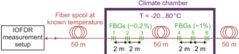
We prepared a sensor fiber, which consisted of the aforemen-tioned FBG arrays spliced to either end of a 50 m HI1060 FLEX single-mode fiber and put it into a climate chamber. Before and after the sensor fiber, a 50 m launch fiber of the same type was used (see Fig. 8). At the end of the fiber chain, a short piece of coreless fiber served as termination.
Initially, the whole setup was left settled at room tempera-ture and a reference measurement was performed. From the acquired reflection/backscatter profile, the connector losses between the fiber segments were determined.
Subsequently, the climate chamber was set to temperatures ranging from−20 to 80◦C in steps of 20 K. For each tem-perature step, the TLS performed a wavelength sweep from 1538 to 1542.5 nm (step size: 20 pm) and the frequency re-sponse of the Rayleigh/FBG channel was measured with the VNA at each wavelength step (see Table 1 for VNA param-eters). From the acquired data set, the spectral shapes of all FBGs were reconstructed (see Fig. 9), the Bragg wavelengths were determined, and the corresponding temperatures were calculated using the calibration curves depicted in Fig. 4.
Figure 10.Temperature measurement results for the lab experi-ment.
were reconstructed applying the inverse fast Fourier trans-form (IFFT) to the frequency response determined at the cor-responding filter bank outputs. Before the calculation of the IFFT, a Blackman window function was applied to suppress unwanted side lobes. From the backscatter profiles, the tem-perature profile was calculated according to Eq. (10).
The room temperature was recorded and the 50 m lead fiber was used to estimate the required calibration coeffi-cientsC1andC2with a least-square-error fit for each mea-surement.
For the FBG reconstruction, the model-based compressed sensing approach (Werzinger et al., 2017) was chosen, which allowed the same modulation bandwidth to be used as for the Raman DTS (only 100 MHz). For the lab measurements, the fiber launch power was approximately 26 dBm.
The results of the FBG and Raman temperature measure-ments are depicted in Fig. 10. A good agreement was found between the temperatures measured with the FBG sensors and the Raman DTS results. In the Raman DTS measure-ments, an average uncertainty better than 1 K (over all cli-mate chamber measurements), a worst-case standard devia-tion of around 2.5 K for the measurement at 80◦C, and on av-erage a standard deviation of 1.5 K was achieved for the sen-sor fiber inside the climate chamber. The 10 to 90 % rise dis-tance was found to be 1.3 m in the 80◦C trace (see Fig. 10).
7 Field test in a high-voltage environment
To verify the functionality of our system under realistic op-erating conditions, we have carried out a field test in a voltage test environment. The device under test was a high-power choke coil made of aluminum with a diameter of around 2.3 m, a height of around 2.9 m, and a nominal induc-tance of 9 mH at operating currents up to 2100 A and voltages up to 15 kV.
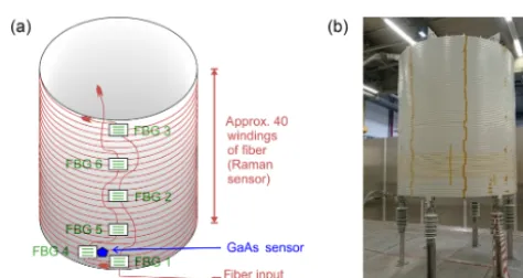
For this experiment, we used the two aforementioned sets of three FBGs and a 300 m long HI1060 Flex single-mode fiber in between (see Fig. 11). The sensor fiber was wound around the coil from top to bottom in around 40 windings and the FBGs were attached vertically at the coil (see Fig. 12).
Figure 11.Fiber configuration for the field test.
Figure 12.Installed fiber at the high-power coil for the high-voltage field test ((a)schematic,(b)picture).
The FBGs were attached to the coil using a heat transfer com-pound in order to assure good thermal contact and minimize the strain on the fiber. Additionally, a commercially avail-able GaAs bandgap temperature sensor was installed close to FBG 4 (see Fig. 12) for comparison.
Compared to the laboratory experiment, the measurement system was slightly modified: the avalanche photodiode de-tectors for the detection of the Raman components were re-placed with more sensitive ones that give a better signal-to-noise ratio and allowed the optical launch power to be re-duced and the VNA parameters to be adjusted (see Table 2) for faster measurements. Moreover, the filter bank was up-graded with two additional filters to further enhance the iso-lation between the Raman and the FBG/Rayleigh channel. This allowed us to average the traces acquired during the wavelength scan over all wavelengths and use them for the Raman DTS. The optical launch power into the sensor fiber was reduced to approximately 23 dBm.
At the beginning of the test, no current was flowing through the coil and it was in a thermal equilibrium at room temperature (approximately 25.5◦C). After switching on, a current of 400 A was flowing in approximately the first 4 min before it was increased to around 975 A within 3 min. After approximately 5 h, the current was switched off and the coil was allowed to cool down again. During the test, the surement setup remained unchanged. The same VNA mea-surement parameter set was used for the determination of the temperatures based on Raman DTS and FBG sensors.
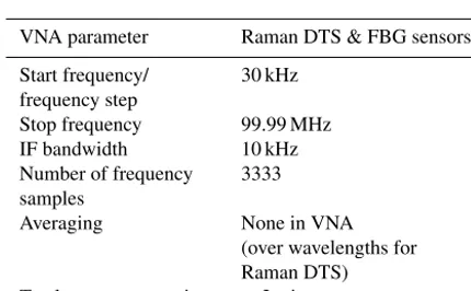
Table 2.VNA measurement parameters for the Raman DTS and FBG temperature sensor measurements in the field test.
VNA parameter Raman DTS & FBG sensors
Start frequency/ 30 kHz frequency step
Stop frequency 99.99 MHz IF bandwidth 10 kHz Number of frequency 3333 samples
Averaging None in VNA (over wavelengths for Raman DTS) Total measurement time ≈2 min
Although the 300 m fiber segment and the 50 m launch fiber were both HI1060 Flex fibers, we found they had differ-ent properties possibly due to aging or batch-to-batch vari-ation, since the 300 m fiber was much older and had been used in many temperature experiments before. Especially the different attenuation of Raman Stokes and anti-Stokes wavelengths is problematic because it skews the ratio pro-fileI0AS(z)/I0S(z). We have therefore used a measurement that was taken before the test when the coil was in thermal equilibrium to determine the tilt resulting from the different attenuation and to compensate for it in all other measure-ments.
The calibration sections to determine the coefficientsC1 andC2in Eq. (9) were a short segment of the 300 m fiber before the coil that was at room temperature and the section at the GaAs temperature sensor.
The resulting temperature distribution for three instances of time mapped onto a cylinder representing the coil is de-picted in Fig. 13. It can be seen that the coil gets warmer at the top and that there is a temperature gradient towards the bottom windings. This is confirmed by an image of the heated coil taken with a thermal camera (see Fig. 14).
Figure 15 represents the temporal change of temperature for three different fiber segments (each averages over two windings of fiber) corresponding to the top, middle, and lower part of the coil. Furthermore, the read-outs of the GaAs
Figure 14.Thermal image of the coil when it was heated up (no temperature calibration due to unknown emissivity).
sensor and the current through the coil are plotted. Interest-ingly, a decrease of the temperature in all segments can be observed between 10 and 11 h. This is probably due to ven-tilation in the test site at that time, which was also observed by the experimenters. The GaAs sensor was attached to the heat transfer compound covered by tape, which probably pre-vented the corresponding spot from cooling down.
The temporal evolution of the measured FBG tempera-tures is depicted in Fig. 16. The temperature of the GaAs sensor before the warm-up is taken as an initial reference for all FBGs. Like the Raman measurement, the temperatures of the FBGs at the top of the coil (FBG 3 and FBG 6) reach the highest temperature (∼46◦C) and there is a decreasing trend towards the bottom (∼ 35◦C). However, the
Figure 15.Temporal change of the temperature measured with Raman DTS at three different locations of the coil (mean of two windings at the top, middle, bottom) and the GaAs sensor measurements for reference.
Figure 16.Temporal change of the temperature measured with the FBGs at six different locations of the coil and the GaAs sensor measure-ments for reference.
mitigated by improved packaging of the FBGs to make sure mechanical stress cannot disturb the measurement.
8 Summary
In this work, we have successfully demonstrated a fiber optical temperature measurement system based on IOFDR, which combines FBG temperature sensors and Raman-based DTS to enable both distinct hot spot and truly distributed temperature profile measurements over a wide range of tem-peratures, with a 10 to 90 % rise distance of around 1 m. We have also demonstrated that there are no general restrictions for using our system in a high-voltage environment.
9 Outlook
Future work is planned to address the electrical components in our system. Instead of a costly and feature-rich vector net-work analyzer, a custom-made solution would be desirable to reduce the system cost, size, and complexity while poten-tially increasing the measurement speed. Furthermore, possi-ble benefits of the combination of the measurement data from Raman DTS and FBGs, such as temperature-compensated strain measurements with FBGs, should be evaluated.
Data availability. The underlying measurement data are not pub-licly available and can be requested from the authors if required.
Competing interests. The authors declare that they have no con-flict of interest.
Special issue statement. This article is part of the special issue “Sensor/IRS2 2017”. It is a result of the AMA Conferences, Nurem-berg, Germany, 30 May–1 June 2017.
Acknowledgements. Parts of this work were funded by the Ger-man Federal Ministry for Economic Affairs and Energy (BmWE) under the grant no. 03ET7522B (project “iMonet”).
We would like to thank the Siemens AG (Nuremberg, Germany) and especially Uemit Genc for the cooperation and the participation in the field test.
Edited by: Werner Daum
Engelbrecht, R.: Stimulierte Raman-Streuung, in: Nichtlineare Faseroptik, Springer, Berlin Heidelberg, Germany, 205–282, https://doi.org/10.1007/978-3-642-40968-4, 2014.
Filho, E., Baiad, M., Gagné, M., and Kashyap, R.: Fiber Bragg grat-ings for low-temperature measurement, Opt. Express, 22, 27681– 27694, https://doi.org/10.1364/OE.22.027681, 2014.
Ghafoori-Shiraz, H. and Okoshi, T.: Optical-fiber diagnosis using optical frequency-domain reflectometry, Opt. Lett., 10, 160–162, 1985.
Harris, F. J.: On the use of windows for harmonic analysis with the discrete Fourier transform, Proc. IEEE, 66, 51–83, https://doi.org/10.1109/PROC.1978.10837, 1978.
Hu, C., Wang, J. Zhang, Z., Jin, S., and Jin, Y.: Application research of distributed optical fiber temperature sensor in power system, Asia Communications and Photonics Conference and Exhibition (ACP), Shanghai, 2011, 1–6, https://doi.org/10.1117/12.905303, 2011.
Iizuka, K., Freundorfer, A. P., Wu, K. H., Mori, H., Ogura, H., and Nguyen, V.-K.: Step-frequency radar, J. Appl. Phys., 56, 2572– 2583, https://doi.org/10.1063/1.334286, 1984.
ence on Sensors and Measurement Technology, edited by: AMA Service GmbH, SENSOR 2017, Nürnberg, 30 May–1 June 2017, AMA Service GmbH, Wunstorf, 261–266, 2017.
Liehr, S., Lenke, P., Wendt, M., Krebber, K., Seeger, M., Thiele, E., Metschies, H., Gebreselassie, B., and Munich, J. C.: Polymer Optical Fiber Sensors for Distributed Strain Measurement and Application in Structural Health Monitoring, IEEE Sens. J., 9, 1330–1338, https://doi.org/10.1109/JSEN.2009.2018352, 2009. Ukil, A., Braendle, H., and Krippner, P.: Distributed Temperature
Sensing: Review of Technology and Applications, IEEE Sens. J., 12, 885–892, https://doi.org/10.1109/JSEN.2011.2162060, 2012.
Werzinger, S., Bergdolt, S., Engelbrecht, R., Thiel, T., and Schmauss, B.: Quasi-Distributed Fiber Bragg Grating Sensing Using Stepped Incoherent Optical Frequency Do-main Reflectometry, J. Lightwave Technol., 34, 5270–5277, https://doi.org/10.1109/JLT.2016.2614581, 2016.
Werzinger, S., Gottinger, M., Gussner, S., Bergdolt, S., Engelbrecht, R., and Schmauss, B.: Model-based compressed sensing of fiber Bragg grating arrays in the frequency domain, Proc. SPIE 10323, 25th International Conference on Optical Fiber Sensors (OFS), Jeju, Korea, https://doi.org/10.1117/12.2263462, 2017.