R E S E A R C H
Open Access
Influence of transect length and downed
woody debris abundance on precision of
the line-intersect sampling method
Shawn Fraver
1*, Mark J. Ducey
2, Christopher W. Woodall
3, Anthony W. D
’
Amato
4, Amy M. Milo
5and Brian J. Palik
6Abstract
Background:Accurate downed woody debris (DWD) volume or mass estimates are needed for numerous applications such as fuel loading, forest carbon, and biodiversity/habitat assessments. The line-intersect sampling (LIS) method of inventorying DWD is widely used in forest inventories and ecological studies because it is time-efficient and unbiased. Despite its widespread use, the appropriate transect length needed to achieve a desired precision at a particular location has received relatively little attention.
Methods:We conducted intensive LIS sampling at 33 locations representing eight mature or old-growth forest types in northeastern USA, providing a range of forest conditions and DWD volumes (from 17 to 323 m3∙ha−1). We used these empirical field data to test, through simulations, the effect of increasing transect length (up to 340 m at each location) on precision of associated LIS volume estimates. Importantly, we used a novel application of copula models to account for within-transect spatial autocorrelation of DWD volumes during our simulations, thereby properly addressing variance estimates.
Results:As expected, precision consistently improved with increasing cumulative transect length, and locations with lower DWD volumes required longer transects to achieve a given level of precision. We developed models relating precision, transect length, and DWD volume that allows us to gauge a suitable LIS transect length for desired precision levels.
Conclusions:LIS provides an attractive method for estimating DWD volume for a given localized area of interest. For the forest types sampled here, and for the particular copula model framework employed, transect lengths of ca. 120 m provide a reasonable level of precision, ranging from 18% to 60% coefficients of variation.
Keywords:Coarse woody debris, Copula model, Dead wood, Fuel loads, Forest structure, Forest carbon
Background
Research over the past decades has clearly established the vital role of downed woody debris (DWD) in forest eco-systems, where it influences biodiversity, nutrient cycling, soil development, and wildfire behavior (Harmon et al.
1986; Schoennagel et al. 2004; Stokland et al. 2012).
Recent attention has shifted to carbon stores and fluxes in DWD given the growing interest in carbon dynamics in
the context of climate change (Russell et al.2014; Woodall
et al.2015). Methods of reliably estimating DWD
abun-dance in forest systems are thus critical for carbon
estimates (e.g. Russell et al. 2015), as well as a broader
range of applications.
As with live-tree sampling, a complete census could be conducted of all DWD pieces above a minimum diam-eter threshold within a location of interest; however, this may be impractical for inventories at stand or larger scales. As a consequence, sampling methods such as line-intersect sampling (LIS) are employed to inventory
DWD abundance (Woodall et al.2009). LIS produces an
area-based estimate of DWD volume derived from a sample of the logs present. In the field, the intersect method proceeds by measuring diameters of pieces (above a given size threshold) at the point where an
in-ventory transect crosses the pieces’central longitudinal
* Correspondence:[email protected]
1School of Forest Resources, University of Maine, Orono, ME, USA Full list of author information is available at the end of the article
axes. The resulting data (tallied diameters and total tran-sect length) are converted to area-based estimates of DWD volume, typically using equations provided by Van
Wagner (1968) and Brown (1974). The theory
under-lying LIS is well developed (de Vries1979; Kaiser1983).
No assumption of piece shape is required, as LIS leads naturally to an unbiased Monte Carlo estimate of vol-ume based on the cross-section of pieces where they are intersected by the transect line. Moreover, despite some derivations that assume pieces are randomly distributed
(e.g. Warren and Olsen 1964), from a design-based
per-spective, the positions of pieces are regarded as fixed even if they originated from a random process. Because it is time-efficient and design-based unbiased, LIS is widely used in ecological studies and fuel inventories (e.g. Brown
1974), as well as in many national-scale forest inventories
(Woodall et al.2009). Kershaw et al. (2016, ch. 12) provide a practical and theoretical review of LIS along with alter-native DWD inventory approaches.
Despite its widespread use in large-scale forest inventor-ies, the appropriate LIS transect lengths needed under local forest settings has received relatively little attention (but see
Woldendorp et al.2004; Sikkink and Keane2008).
Consid-ering that many ecological studies intend to characterize DWD attributes at particular locations, where forest stands or small reserves are themselves the populations of interest
(Jönsson et al. 2011; Fraver and Palik 2012), surprisingly
few studies have evaluated DWD sampling methods at this
local scale. Stokland et al. (2004) caution that a DWD
sam-pling design that is efficient for assessing average ecological values over large scales may be poorly matched to the task of assessing those same values at local scales.
Previous empirical work as well as sampling theory demonstrates that for a given site the precision of the LIS estimate consistently improves (lower variance) with in-creasing cumulative transect length (Pickford and Hazard
1978; Woldendorp et al.2004; Miehs et al.2010) and that
sites with lower DWD volume generally require longer transects to achieve a desired level of precision (Brown
1974; Pickford and Hazard1978; Woldendorp et al.2004).
The objective of the present study was two-fold: 1) to better quantify the effect of increasing transect length and DWD volumes on the precision of LIS volume esti-mates, and 2) to provide practical guidance for selecting transect lengths that achieve a desired level of precision regarding LIS volume estimates. We addressed these objectives through simulations constrained by empirical LIS data from 33 locations representing eight diverse forest types in the northeastern USA. These locations provide a range of forest conditions and DWD volumes, making them ideal for addressing these objectives. Additionally, we present a novel application of copula models to account for within-transect spatial autocorrel-ation of DWD volumes; without accounting for such
autocorrelation, simulations would underestimate the variance within transects, resulting in spurious assess-ments of appropriate transect lengths.
Methods
Study locations and field data collection
We tested the effect of increasing transect length (up to ca. 340 m) and DWD volume on LIS precision using 33 locations representing eight mature or old-growth forest
types in northeastern USA (Table1). These forest types
and locations were utilized opportunistically, given that we needed DWD inventories for these locations as part
of on-going research (e.g., Fraver and Palik2012; Fraver
et al. 2017). We thus opted to intensify sampling (i.e.,
long transects) to provide data for the modelling efforts presented here. These locations represent diverse forest compositions and structures, and they conveniently capture a large range of DWD volumes necessary for
modelling. Forest types include mature red-spruce (Picea
rubens), mature spruce–hemlock (P. rubens,Tsuga cana-densis), mature hemlock–pine (T. canadensis, Pinus strobus), mature mixed conifer–hardwood (T. canadensis, Acer saccharum, Fagus grandifolia, Betula alleghaniensis),
mature northern hardwoods (A. saccharum, F.
grandi-folia, B. alleghaniensis, with P. rubens), old-growth
northern white-cedar (Thuja occidentalis), old-growth
red pine (Pinus resinosa), and old-growth black ash
(Fraxinus nigra). A minimum of three locations was established in each forest type. Additional site
infor-mation is provided in Table 1.
At each location we conducted LIS sampling using a cluster of four transects that intersected at their midpoints as follows: two diagonal 100-m transects (arranged south-west to northeast and northsouth-west to southeast) and two 70-m transects (arranged in cardinal directions). This
configuration formed a spoke-like‘union jack’with equal
angles between transects and a total transect length of 340 m. At four of the eight sites, the centers of the union jacks were placed on centers of existing long-term con-tinuous forest inventory plots. At the remaining four sites, where previous plots did not exist, centers were placed randomly within sampled stands. This union jack config-uration was initially employed at the red-pine locations
(the first to be sampled; Fraver and Palik2012), as an
ex-ploratory comparison of co-located LIS and fixed area in-ventories on 0.5-ha (70.7 m × 70.7 m) plots (unpublished). For sampling consistency, we then used this same config-uration at all remaining locations. A multi-directional, spoke-like arrangement is often used to reduce potential sample variance when DWD pieces exhibit fairly uniform
fall directions (Van Wagner 1968). The most common
random, these equations provide unbiased estimates, but
strong correlation in the pieces’fall directions can inflate
sample variance (Kaiser1983; Kershaw et al.2016, ch. 12).
Spoke-like transect designs have been the subject of some
debate in large-area inventories (Affleck et al. 2005; but
see Woodall and Monleon2008); however, their use
rep-resents common field practice (e.g., Dunn and Bailey
2015), and we feel the design is adequate to evaluate the
effect of varying transect lengths, the focus of our study. For each DWD piece intersected by the sampling transect
with a diameter≥10 cm at the intersection, we recorded
diameter at intersection, distance from center, species, and
decay class (five-class system as per Sollins 1982). By
convention, if a piece intersected two transects, or if it crossed the same transect twice, it was recorded
twice (Van Wagner 1968, Brown 1974).
We calculated DWD volume for each site as follows,
V¼ π2Xd
2
8L
10 000
where V is the area-based volume (m3∙ha−1), d is the DWD piece diameter (m) at point of intersection, andLis the total transect length at the site (m) (from Van Wagner 1968). Similar calculations were used to provide volume es-timates for short 5-m segments of each transect, to be used in the sampling simulations described below.
Simulation of sampling variability
To assess how transect length and population character-istics influence sampling variability, we employed a model-based approach using simulation based on a zero-inflated, autoregressive copula. To motivate this approach, let us first consider a naive approach that would be simple to implement, and would have some desirable features, but could lead to inaccurate results. Given the line intersect data from a site, with the positions of all the intersections recorded, one could subdivide
transects into shorter segments (e.g., 5 m) that would allow simulation of the sampling variance for different transect lengths, with a resolution on length that would be meaningful for operational inventory design. Then, to simulate transects of different total length, one would draw segments at random with replacement from the data for that site, concatenating them to form transects of the desired length. For example, to form a 20-m transect, one would choose four segments of 5 m each with replace-ment, and compute any desired values (such as DWD volume) for the new, simulated transect. By repeating this process many times, and varying the transect length, one would develop a Monte Carlo estimate of the sampling distribution of DWD volume estimates for LIS at that site and its dependence on transect length, with a richer potential inference beyond
second-order statistics such as variance (which,
under the assumptions implicit in this approach, could also be calculated using the usual formulae for
simple random sampling; e.g., Thompson 2012).
Es-sentially, this approach uses the same rationale as
the bootstrap (Efron and Tibshirani 1993),
substitut-ing the empirical distribution of DWD volume on short segments for the unknown population distribu-tion of possible segments, to arrive at the sample dis-tribution through resampling.
Unfortunately, the bootstrap approach makes a strong independence assumption that is inappropriate for DWD data under either a design- or model-based ap-proach (for details on the distinction, see Gregoire
1998). Within a design-based framework (Kaiser 1983;
Gregoire and Valentine2008), DWD pieces are fixed but
sample selection is random. The entire transect is a single randomly selected sample unit, and treating segments within a sample unit as if they were drawn in-dependently is anathema. Without substantial additional information (such as the joint inclusion probabilities of the individual pieces of DWD) it is difficult to make Table 1Characteristics of the eight forest types from which empirical data were collected for evaluation of LIS precision
Site Forest type No. locations Mean (range)
DWD vol. (m3∙ha−1)
Howland Forest, Maine Spruce-hemlock 3 25 (17–36)
BBEW, Maine Northern hardwoods 4 46 (32–61)
PEF, Maine Hemlock-white pine 3 52 (35–66)
Baxter SFMA, Maine Red spruce 3 55 (42–70)
Various, Minnesota Red pine 7 81 (51–137)
BEF, New Hampshire Mixed conifer-hardwood 3 84 (58–111)
Various, Minnesota Black ash 6 126 (70–243)
BRFR, Maine Northern white-cedar 4 258 (205–323)
progress from this perspective, beyond inference based on the design that was actually employed (except for changes in the number, rather than the length, of sample tran-sects). While a design-based approach has substantial benefits, both in terms of formulating a design for a specific inventory, and computing defensible estimates once the data are in hand, to understand how differ-ent designs (such as varying transect lengths) would impact estimates and their uncertainty, a model is in-valuable. However, from a model-based perspective, the independence of short, contiguous segments is also suspect. One might expect positive autocorrel-ation of the values from adjacent segments, not only because of the potential for spatially clumped inputs from tree mortality, but also because local terrain might cause DWD pieces that are close to each other also to share similar orientation. In the presence of positive autocorrelation, the variance of estimates from transects of a given length would be higher than that implied by independent segments, and the tran-sect length needed to reach a given level of accuracy would be longer. To summarize: from a design-based perspective, successive segments within a randomly selected transect are likely to display autocorrelation because of the fixed characteristics of the downed woody debris population. From a model-based perspective, the in-dependence of successive short segments is also suspect, because of likely clumping in the random process that generates the population. Whichever perspective is taken in inference, it would appear important to in-corporate autocorrelation within any simulations.
To address the challenge of autocorrelation among successive segments, while remaining faithful to the observed marginal distribution of estimates from those segments, we employ a copula modeling approach. Within the forestry literature, we believe this is the first application to employ an autoregressive model (to account for correlation between successive segments), and also to address a zero-inflated distribution (many segments are empty, with no DWD intersections). Copula models are relatively new in the forestry litera-ture; they have been used to describe relationships be-tween continuous variables such as tree diameter and
height (Wang et al. 2008, 2010; MacPhee et al.2017),
to inform spatially-explicit stand simulations (Kershaw
et al. 2010), and for imputation-based growth and
yield models (Kershaw et al. 2017). Eskelson et al.
(2011) and Fortin et al. (2013) extended copula models
in forestry to account for spatial autocorrelation. More re-cently, copula methods have been used to simulate spatial populations for remote sensing-assisted inventory (Ene et al.2012,2013a,2013b; Grafström et al.2014). For a some-what theoretical overview of copulas, see Genest and Mac-kay (1986) and Nelsen (2006).
Strictly defined, a bivariate copula describes the
rela-tionship between two random variablesxand yin terms
of two random deviates that are uniformly distributed
on [0, 1]. Specifically, if U1 and U2 ~ Uniform (0, 1),
then the copulaCis defined as
C uð 1;u2Þ ¼ PrfU1≤u1;U2≤u2g
IfFX(x) andFY(y) are the cumulative distribution
func-tions ofxandy, then
FXYðx;yÞ ¼C Fð Xð Þx ;FYð Þy Þ
In our application, x andy are the volume estimates
(m3∙ha−1) associated with successive pairs of short
LIS segments within the same dead wood population; thus, they share the same cumulative distribution function F(x) =FX(x) =FY(y). A variety of formulations
have been proposed to model the copula function C.
For simulation purposes, one of the simplest is the
Gaussian or normal copula (Wang1998). LetZ1andZ2
have a standard normal marginal distribution, i.e.,Z1and
Z2~N(0, 1), with correlation coefficientρ. LetΦ(∙) be the cumulative distribution function of the standard normal distribution. Then Φ(Z1) and Φ(Z2) will be bivariate uni-form, with Kendall’s τ= (2/π)acrsin(ρ). More generally, if we simulate a sequence ofZi,i= 1,…,m, the sequence will
be a first-order autoregressive [AR(1)] time series, and each pairΦ(Z1),Φ(Zi +1) will be described by the same copula
functionC. To complete a simulation of a single transect
composed ofm segments, each having marginal
distribu-tionF(x), we employ the following algorithm:
1) Generate a standard normal AR(1) time series of lengthm, with correlation coefficientρ. This can easily be done through the sequential generation of independent random deviates, with appropriate summation to generate successive entries in the time series.
2) Convert the resulting series to an autocorrelated series of uniform deviatesui=Φ(Z1).
3) Apply the inverse of the empirical cumulative distribution function to translate the uniform series to the marginal distribution of downed wood volume estimates,xi=F−1(ui).
The only slight complication in the simulation phase of our application arises due to the zero-inflated nature
of DWD volume data. Specifically, letp0be the
probabil-ity of obtaining xi= 0 in a given population. Then, in
step 3 above,xi= 0 wheneverui<p0.
parameter ρ. In the absence of zero-inflation, the Zi,
ui, and xi would share a common value of Kendall’s
τ (or Spearman’s rank-correlation coefficient), both of
which share a one-to-one relationship with ρ. Thus, it
would be possible to calculate a reasonable value of ρ
based on the value ofτcalculated from the sample pairs
xi, xi+ 1 in the transects for a given population.
Alternatively, one could reverse the process used in simu-lation: calculateui=F(xi) to translate the sample series to
an autocorrelated uniform series, then Zi=Φ−1(ui) to
obtain a standard normal AR(1) series, and finally
estimate ρ from the serial correlation of the Zi.
How-ever, this approach fails for zero-inflated data, because
it is unclear what value to assign to ui (and hence Zi)
when xi= 0.
To overcome this challenge, we adopted a
maximum-likelihood approach based on the estimation of correlation coefficients in the presence of censoring, as originally developed by Lyles et al. (2001). In fact, our situ-ation is somewhat simpler than that described by Lyles et al. (2001), because theZiare defined to have standard
nor-mal distribution; we do not need to concern ourselves with the mean and variance as nuisance parameters.
We reverse-engineer the Zi values as described above,
but record the values as censored whenever xi= 0;
that is, we only know that Zi≤Φ−
1
(p0). Then, we may recognize four distinct categories of outcomes for Zi, Zi+ 1 pairs:
Category 1:In this category, neitherZinorZi+ 1are censored. Pairs of this type contribute lnf(Zi,Zi+ 1) = ln
f(Zi+ 1|Zi) + lnf(Zi) to the log-likelihood. Following Lyles
et al. (2001), we denote this contribution as ln(ti1):
lnð Þ ¼ti1 − 1 2 1ð −ρ2Þ Z
2
iþZ2iþ1−2ρZiZiþ1
− ln 2 π1−ρ2
Category 2:In this category,Ziis known butZi+ 1is censored. LetZ'=Φ−1(p0). The contribution of these pairs to the log-likelihood is
lnð Þ ¼ti2 ln Pr Ziþ1≤Z
0 jZi
h i
þ lnf Zð Þi
which equals
lnð Þ ¼ti2
Z2 i
2 − ln 2ð Þ þπ lnΦ
Z0ffiffiffiffiffiffiffiffiffiffi−Zi 1−ρ2 p
" #
Category 3:In this category,Zi+ 1is known butZiis
censored; by the same rationale as Category 2, the contribution to the log-likelihood is
lnð Þ ¼ti3
Z2iþ1
2 − ln 2ð Þ þπ lnΦ
Z0−ffiffiffiffiffiffiffiffiffiffiZiþ1 1−ρ2 p
" #
Category 4:In this category, bothZiandZi+ 1are censored. Then the contribution to the log-likelihood is ln{Pr[(Zi≤Z')∩(Zi+ 1≤Z')]}, i.e.
lnð Þ ¼ti4 ln 1 ffiffiffiffiffiffi 2π
p
Z Z0
−∞ Φ
Z0−Z
ffiffiffiffiffiffiffiffiffiffi 1−ρ2 p
" #
exp Z
2
2 dZ
( )
Unfortunately, the integral has no convenient, closed-form expression, but it yields readily to numerical integration. By summing the contributions to the log-likelihood across all unique adjacent pairs of seg-ments within a site, one obtains the log-likelihood
func-tion; maximization with respect toρyields the maximum
likelihood estimate, and the inverse of the negative of its second derivative provides the asymptotic variance of the estimate, from which the standard error and confidence limits may be computed.
To summarize: For each location, we used all unique pairs of adjacent 5-m segments, and estimated a
site-specificρand its standard error by maximum
likeli-hood. Then, we simulated artificial transects of varying length using a zero-inflated autogressive copula, based
on the estimated value of ρ and the empirical
distribu-tion of volume estimates for 5-m segments from that location. We simulated transect lengths from 20 m to 340 m by 20-m intervals, with 1000 simulated replica-tions at each length for each location. For comparison
purposes, we performed identical simulations withρ= 0,
i.e., no autocorrelation, for each location. In this case, the simulation is mathematically identical to the inde-pendent bootstrap approach. We summarized the distri-butional characteristics of the 1000 replicates and used the results as response variables for further modeling to characterize the dependence of sampling variability on transect length and DWD volume.
Modeling of simulation results
a standard deviation, calculated from the 1000 runs unique to each transect length–location combination. We used linear and non-linear mixed-effects models to evaluate the influence of transect length and total DWD volume (pre-dictor variables, unique to each location) on the coefficient of variation (CV) of these estimates. Total DWD volume refers to that calculated from the full 340-m transect length for each location. We first tested the predictors in individ-ual models and then combined them to determine the best-fit two-term model. Forest type was included as a random factor in all models, given that we are not making inferences about particular forest types, for which our sam-ple size (3–7 locations per type) is inadequate. Logarithmic and square-root transformations of response and pre-dictor variables were explored for stabilizing variance and improving residual-versus-predicted diagnostics. The fact that our candidate models included trans-formed and non-transtrans-formed variables limited our reliance on Akaike’s information criterion (Burnham and
Anderson 2002) for evaluating model performance.
In-stead, we relied on pseudoR2(see below) and root mean
square error (RMSE, back transformed as needed) values, as well as graphs of observed-versus-predicted and residual-versus-predicted values to determine which models were best supported by the data. For the one-term models, we tested linear, negative exponential, and power function model forms; for the two-term model, we tested linear, negative exponential, power, quadratic, and partial quadratic forms. Analyses were conducted
in thenlmepackage (Pinheiro et al.,2016) in R (version
3.0.3; Core Team, 2016), using the weighting option to
compensate for non-homogenous variance.
Goodness-of-fit (pseudo R2) for the models was expressed as the
correlation between observed and predicted CVs (cf.
Canham et al. 2004).
Results
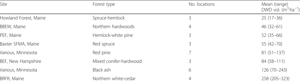
Simulations of various transect lengths revealed that, as expected, the precision (here, CV) of the LIS estimate consistently improved with increasing cumulative tran-sect length. Model comparisons revealed that the rela-tionship between CV and transect length was best
described by a power function (P< 0.0001, R2= 0.801,
RMSE = 0.127) as shown in Fig.1. Importantly, our analysis
of DWD values along transects indicated the presence of spatial autocorrelation, with correlation coefficients (one for each of 33 locations) forming a bimodal distribution; that is, some locations showed positive and others negative autocorrelation (Fig.2).
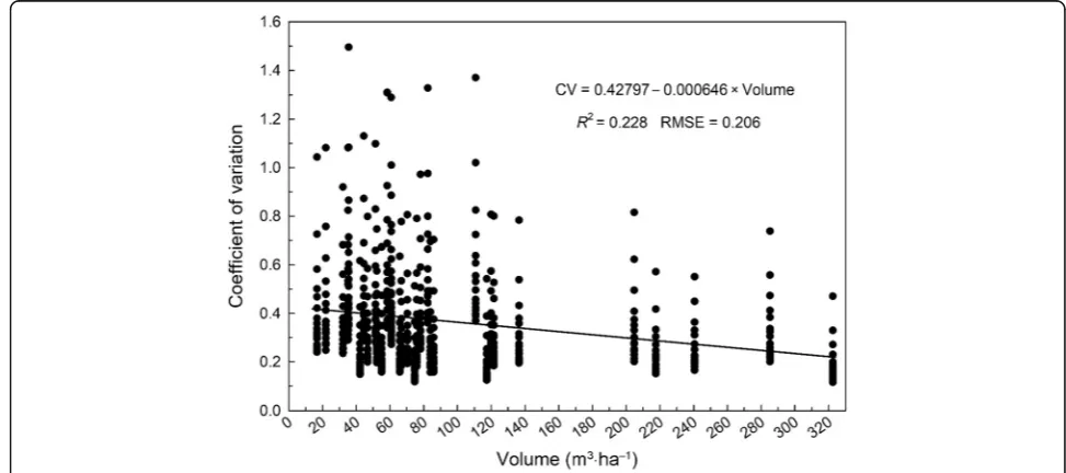
Simulations also revealed that precision of the LIS es-timate improved with increasing DWD volume present, meaning that for a given transect length, greater preci-sion could be achieved where higher DWD volumes are encountered. The relationship between CV and DWD volume was best described by a linear function, as
shown in Fig. 3. Although this model was statistically
significant (P< 0.01), the relationship is quite weak
(R2= 0.228, RMSE = 0.206).
When the CV was modeled as a function of both tran-sect length and DWD volume, model comparisons re-vealed that the exponential relationship was best supported by the data, expressed as CV =a×eb× volume×ec× sqrt_length,
Fig. 1Modelled relationship (black line, accounting for spatial auto-correlation) between line intersect sampling precision (expressed as
where sqrt_length is the square root of transect
length (Fig. 4). However, diagnostics for this model
were poorer than those for the length-only model
(here, R2= 0.795, RMSE = 0.128), and the volume
term became non-significant. For this reason, the length-only model was used for inferences regarding appropriate transect lengths.
Discussion
Our study was motivated by the need to provide guid-ance in selecting a LIS transect length appropriate for estimating DWD volumes for particular locations of interest. We note that a sampling design efficient for assessing average ecological values of DWD over large scales (as in national forest inventories) may not be well
suited for assessing those same values at local scales, such
as small forest reserves (Stokland et al.2004), where the
reserve itself may be the population of interest.
Our finding that the precision of LIS estimates consist-ently improved with increasing transect length corroborates a number of previous studies from quite different forest
types (e.g., Van Wagner 1982; Pickford and Hazard 1978;
Fig. 2Frequency distribution ofρcoefficients for the 33 locations,
suggesting tendencies toward both negative and positive spatial autocorrelation of DWD values within sampling transects
Fig. 3Relationship between line intersect sampling precision (expressed as coefficient of variation) and downed woody debris (DWD) volume.
For a given transect length, sites with greater volumes generally produce more precise estimates
Fig. 4Modelled relationship between line intersect sampling
precision (expressed as coefficient of variation), transect length, and downed woody debris (DWD) volume, using simulations constrained by empirical field data from 33 locations within eight forest types of northeastern USA. Top model form: CV = 1.30268 ×e–0.0002277 × volume
×e–0.1059549 × sqrt_length, where sqrt_length is the square root of
transect length. Diagnostics for this model (R2= 0.795, RMSE = 0.128)
Woldendorp et al.2004; Miehs et al.2010; Keane and Gray
2013). Similarly, our finding that precision of LIS
esti-mates improved with increasing DWD volume present has been reported from a range of distinct forest
systems (Brown 1974; Pickford and Hazard 1978;
Woldendorp et al. 2004). However, the best-fit model
that included both transect length and DWD volume as predictors showed poorer diagnostics than that of the length-only model described above, suggesting that the
length-only model (shown in Fig. 1) could be used for
inferences regarding appropriate transect lengths.
If DWD pieces were distributed at random, basic
sampling theory (e.g. Thompson 2012) predicts that the
variance of the total DWD intersected by a transect would scale linearly with transect length; thus, the CV
would scale with the−0.5 power of transect length for a
given DWD density. However, clumping or regularity in DWD pieces would produce a departure from this scal-ing relationship. Indeed, our analysis of DWD values along transects revealed the presence of spatial autocor-relation, with some locations tending toward positive
and others toward negative autocorrelation (Fig.2). We
found no discernable pattern among locations regard-ing forest type or DWD volume that might explain the bimodal distribution. We minimized the confounding effects of autocorrelation through simulations based on a zero-inflated autoregressive copula model, which accounted for correlations between adjacent 5-m tran-sect segments unique to each location. Without ac-counting for such autocorrelation, our simulations
would have underestimated variance (Fig. 1), leading to
spurious assessments of appropriate transect lengths. To the best of our knowledge, this is the first attempt to employ an autoregressive model to account for spatial autocorrelation, while also addressing a zero-inflated dis-tribution (segments may contain no DWD).
A frequent question in the design of research or moni-toring protocols is how long transects should be to pro-vide a reliable DWD volume estimate for a given location. A perusal of literature where LIS was used to estimate DWD volume for particular locations reveals substantial variation in the transect length employed: total transect lengths can range from < 40 m (Bradford and Kastendick
2010; Buma et al. 2014) to 200 m or more (Ekbom et al.
2006; Lõhmus and Kraut 2010). For the forest types and
conditions sampled here, and considering the particular copula model framework employed, transect lengths of ca. 120 m provide what we feel is a reasonable level of preci-sion, ranging from 18% to 60% CV from the observed sim-ulations, and 37% from the fitted model results, across the
range of DWD volumes encountered (Fig.1). Practitioners
working in these or similar forest types and requiring greater precision could chose a transect length based on
the curve or equation presented in Fig. 1. For our own
inventories, we find it convenient to arrange three 40-m transects radiating equi-angularly from a center point. This total length is somewhat comparable to the 100 m
recommended by Woldendorp et al. (2004) for eucalypt
forests of Australia to remain below a 100% CV threshold. Regarding the national DWD inventory of the US
(Woodall and Monleon 2008), the total transect length
sampled in a fully forested plot is 88 m, which would place the estimated CV below 43% for the locations sampled here. This level of uncertainty may be accept-able, as the strategic-scale inventory is designed to pro-duce reliable DWD estimates (e.g., CV’s below 10%) at the scale of entire forest types or regions (Woodall et
al. 2013), not for particular locations of interest, the
focus of our study.
LIS provides an attractive method for estimating DWD volume for a given localized area of interest, particularly when transects of reasonable length are employed. LIS sampling has been repeatedly shown to be much more time efficient than the other common sampling
alterna-tive, namely censuses of fixed area plots (Bailey 1970;
Jordan et al. 2004). Nevertheless, a complete census of
large plots, including mapping of DWD pieces, may re-main the method of choice in studies where spatial information is needed, or where a particular plot size is needed for comparability to preexisting benchmarks
(see Rouvinen and Kouki 2002; Jönsson et al. 2008).
It should not be assumed, however, that a complete census of a large plot yields a precise estimate of DWD volume, in part because of the chance of overlooking hard-to-detect
DWD pieces (Jordan et al.2004; Kershaw et al.2016), and
more importantly because of the bias inherent in an
as-sumed piece shape (Fraver et al. 2007; Ducey and Fraver
2018), both problems against which LIS provides natural
safeguards. That is, LIS requires tallying only those pieces that cross a specific, well-defined transect, thus avoiding the need to search a large area for hard-to-detect pieces, and as above, no assumption of piece shape is required for LIS sampling.
Conclusions
to account for within-transect spatial autocorrelation of DWD volumes during our simulations, while also ad-dressing a zero-inflated distribution (transect segments may contain no DWD), thereby properly addressing variance estimates. As expected, precision of DWD vol-ume estimates improved dramatically with increasing cumulative transect length; precision improved only slightly with increasing DWD volumes. For the forest types sampled here, as well as the particular copula model framework employed, transect lengths of ca. 120 m provide a reasonable level of precision, ranging from 18% to 60% coefficients of variation. Finally, we note that although we have focused our analyses on DWD volume, these same results would apply to estimates of DWD biomass or carbon density, as these are typically calculated directly from volume data.
Abbreviations
AR:Auto-regressive; CV: Coefficient of variation; DWD: Downed woody debris; LIS: Line-intersect sampling
Acknowledgements
We thank Aakala T, Clark J, Curzon M, Doud E, Fien E, Foster J, Gill K, Kilbride J, Klockow P, Kuehne C, Manley H, Reinikainen M, Souder C, and Teets A for assistance in the field or laboratory. We thank Russell M, Sikkink P, and Stanovick J for thoughtful comments on earlier drafts of the manuscript. We thank the many staff and scientists at the Penobscot Experimental Forest, Bartlett Experimental Forest, Howland Research Forest, Bear Brook Experimental Watershed, The Northeast Wilderness Trust, The Nature Conservancy, and Baxter State Park Scientific Forest Management Area for maintaining these sites and facilitating our field research.
Funding
Support was provided by the Maine Agricultural and Forest Experiment Station, the Joint Fire Science Program (Project 08–1–5-04), and the USDA Forest Service Northern Research Station.
Availability of data and materials
The materials described in the manuscript including all relevant raw data will be freely available upon request from the corresponding author.
Authors’contributions
SF conceived and designed the study, conducted/supervised the field inventory, and led the analyses of simulation results. MD conceived, conducted, and wrote text addressing the copula models. SF and MD drafted the first version of the manuscript. CWW and AWD assisted with interpretation of results and contributed to writing. All authors contributed to editing and revising the final manuscript. All authors read and approved the final manuscript.
Ethics approval and consent to participate Not applicable.
Competing interests
The authors declare that they have no competing interests.
Author details
1School of Forest Resources, University of Maine, Orono, ME, USA. 2Department of Natural Resources and the Environment, University of New Hampshire, Durham, NH, USA.3US Forest Service, Northern Research Station, Durham, NH, USA.4Rubenstein School of Environment and Natural Resources, University of Vermont, Burlington, VT, USA.5Department of Biological Sciences, George Washington University, Washington, DC, USA. 6US Forest Service, Northern Research Station, Grand Rapids, MN, USA.
Received: 30 April 2018 Accepted: 5 November 2018
References
Affleck DLR, Gregoire TG, Valentine HT (2005) Design unbiased estimation in line intersect sampling using segmented transects. Environ Ecol Stat 12(2):139–154 Bailey GR (1970) A simplified method of sampling logging residue. Forest Chron
46(4):288–303
Bradford JB, Kastendick DN (2010) Age-related patterns of forest complexity and carbon storage in pine and aspen–birch ecosystems of northern Minnesota, USA. Can J For Res 40:401–409
Brown JK (1974) Handbook for inventorying downed woody material. USDA For Serv Gen Tech Rep INT-16, Ogden
Buma B, Poore RE, Wessman CA (2014) Disturbances, their interactions, and cumulative effects on carbon and charcoal stocks in a forested ecosystem. Ecosystems 17(6):947–959
Burnham KP, Anderson DA (2002) Model selection and multimodal inference: a practical information-theoretic approach. Springer-Verlag, Inc., New York Canham CD, LePage PT, Coates KD (2004) A neighborhood analysis of canopy tree
competition: effects of shading versus crowding. Can J For Res 34:778–787 Core Team R (2016) R: a language and environment for statistical computing. R
Foundation for Statistical Computing, Vienna, Austria
de Vries PG (1979) Line intersect sampling–statistical theory, applications, and suggestions for extended use in ecological inventory. In: Cormack RM, Patil GP, Robson DS (eds) Sampling biological populations. International Cooperative Publishing House, Fairland
Ducey MJ, Fraver S (2018) The conic-paraboloid formulae for coarse woody material volume and taper and their approximation. Can J For Res 48:966–975 Dunn CJ, Bailey JD (2015) Modeling the direct effects of salvage logging on
long-term temporal fuel dynamics in dry-mixed conifer forests. For Ecol Manag 341:93–109
Efron B, Tibshirani RJ (1993) An introduction to the bootstrap. Chapman & Hall, New York
Ekbom B, Schroeder LM, Larsson S (2006) Stand specific occurrence of coarse woody debris in a managed boreal forest landscape in Central Sweden. For Ecol Manag 221:2–12
Ene LT, Næsset E, Gobakken T (2013a) Model-based inference for k-nearest neighbours predictions using a canonical vine copula. Scand J For Res 28: 266–281
Ene LT, Næsset E, Gobakken T, Gregoire TG, Ståhl G, Holm S (2013b) A simulation approach for accuracy assessment of two-phase post-stratified estimation in large-area LiDAR biomass surveys. Remote Sens Environ 133:210–224 Ene LT, Næsset E, Gobakken T, Gregoire TG, Ståhl G, Nelson R (2012) Assessing
the accuracy of regional LiDAR-based biomass estimation using a simulation approach. Remote Sens Environ 123:579–592
Eskelson BNI, Madsen L, Hagar JC, Temesgen H (2011) Estimating riparian understory vegetation cover with beta regression and copula models. For Sci 57:212–221
Fortin M, Delisle-Boulianne S, Pothier D (2013) Considering spatial correlations between binary response variables in forestry: an example applied to tree harvest modeling. For Sci 59(3):253–260
Fraver S, Dodds K, Kenefic LS, Morrill R, Seymour RS, Sypitkowski E (2017) Forest structure following tornado damage and salvage logging in northern Maine, USA. Can J For Res 47:560–564
Fraver S, Palik BJ (2012) Stand and cohort structures of old-growthPinus resinosa -dominated forests of northern Minnesota, USA. J Veg Sci 23:249–259 Fraver S, Ringvall A, Jonsson BG (2007) Refining volume estimates of down
woody debris. Can J For Res 37:627–633
Genest C, MacKay J (1986) The joy of copulas: bivariate distributions with uniform marginals. Am Stat 40:280–283
Grafström A, Saarela S, Ene LT (2014) Efficient sampling strategies for forest inventories by spreading the sample in auxiliary space. Can J For Res 44: 1156–1164
Gregoire TG (1998) Design-based and model-based inference in survey sampling: appreciating the difference. Can J For Res 28:1429–1447
Gregoire TG, Valentine HT (2008) Sampling strategies for natural resources and the environment. Chapman & Hall/CRC, New York
Jönsson M, Fraver S, Jonsson BG (2011) Spatio-temporal variation of coarse woody debris input in woodland key habitats in Central Sweden. Silva Fenn 45(5):957–967
Jönsson MT, Edman M, Jonsson BG (2008) Colonization and extinction patterns of wood-decaying fungi in a boreal old-growthPicea abiesForest. J Ecol 96: 1065–1075
Jordan GJ, Ducey MJ, Gove JH (2004) Comparing line-intersect, fixed-area, and point relascope sampling for dead and downed coarse woody material in a managed northern hardwood forest. Can J For Res 34:1766–1775 Kaiser L (1983) Unbiased estimation in line-intercept sampling. Biometrics 39:
965–976
Keane RE, Gray K (2013) Comparing three sampling techniques for estimating fine woody down dead biomass. Int J Wildland Fire 22(8):1093–1107 Kershaw JA, Weiskittel AR, Lavigne MB, McGarrigle E (2017) An imputation/
copula-based stochastic individual tree growth model for mixed species Acadian forests: a case study using the Nova Scotia permanent sample plot network. Forest Ecosystems 4(1):15.https://doi.org/10.1186/s40663-017-0102
Kershaw JA Jr, Ducey MJ, Beers TW, Husch B (2016) Forest Mensuration, 5th edn. Wiley, New York
Kershaw JA Jr, Richards EW, McCarter JB, Oborn S (2010) Spatially correlated forest stand structures: a simulation approach using copulas. Comput Electron Agric 74:120–128
Lõhmus A, Kraut A (2010) Stand structure of hemiboreal old-growth forests: characteristic features, variation among site types, and a comparison with FSC-certified mature stands in Estonia. For Ecol Manag 260(1):155–165 Lyles RH, Williams JK, Chuachoowong R (2001) Correlating two viral load assays
with known detection limits. Biometrics 57:1238–1244
MacPhee C, Kershaw JA, Weiskittel AR, Golding J, Lavigne MB (2017) Comparison of approaches for estimating individual tree height–diameter relationships in the Acadian forest region. Forestry 91:132–146
Miehs A, York A, Tolhurst K, Di Stefano J, Bell T (2010) Sampling downed coarse woody debris in fire-prone eucalypt woodlands. For Ecol Manag 259:440–445 Nelsen RB (2006) An introduction to copulas, 2nd edn. Springer, Inc. New York,
p 272
Pickford SG, Hazard JW (1978) Simulation studies on line intersect sampling of forest residue. For Sci 24(4):469–483
Pinheiro J, Bates D, DebRoy S, Sarkar D (2016) Nlme: linear and nonlinear mixed effects models. CRAN. R-package. R Foundation for Statistical Computing, Vienna
Rouvinen S, Kouki J (2002) Spatiotemporal availability of dead wood in protected old-growth forests: a case study from boreal forests in eastern Finland. Scand J Forest Res 17:317–329
Russell M, Fraver S, Aakala T, Gove J, Woodall CW, D’Amato AW, Ducey MJ (2015) Quantifying carbon stores and decomposition in dead wood: a review. For Ecol Manag 350:107–128
Russell MB, Woodall CW, D’Amato AW, Fraver S, Bradford JB (2014) Technical note: linking climate change and downed woody debris decomposition across forests of the eastern United States. Biogeosciences 11:6417–6425 Schoennagel T, Veblen TT, Romme WH (2004) The interaction of fire, fuels, and
climate across Rocky Mountain forests. Bioscience 54:661–676
Sikkink PG, Keane RE (2008) A comparison of five sampling techniques to estimate surface fuel loading in montane forests. Int J Wildland Fire 17:363–379 Sollins P (1982) Input and decay of coarse woody debris in coniferous stands in
western Oregon and Washington. Can J For Res 12:18–28
Stokland JN, Siitonen J, Jonsson BG (2012) Biodiversity in dead wood. Cambridge University Press, Cambridge
Stokland JN, Tomter SM, Söderberg U (2004) Development of dead wood indicators for biodiversity monitoring: experiences from Scandinavia. In: Marchetti M (ed) Monitoring and indicators of forest biodiversity in Europe– from ideas to operationality. European Forest Institute proceedings 51, Joensuu, Finland, pp 207–226
Thompson SK (2012) Sampling, 3rd edn. John Wiley & Sons, New York Van Wagner CE (1968) The line intersect method in forest fuel sampling. For Sci
14(1):20–26
Van Wagner CE (1982) Practical aspects of the line intersect method, vol 12. Petawawa National Forestry Institute, Chalk River
Wang M, Rennolls K, Tang S (2008) Bivariate distribution modeling of tree diameters and heights: dependency modeling using copulas. For Sci 54:284–293 Wang M, Updhyay A, Zhang L (2010) Trivariate distribution modeling of tree
diameter, height, and volume. For Sci 56:290–300
Wang SS (1998) Aggregation of correlated risk portfolios: models and algorithms. Proc Casualty Actuarial Soc 85:848–937
Warren WG, Olsen PF (1964) A line intersect technique for assessing logging waste. For Sci 10:267–276
Woldendorp G, Keenan RJ, Barry S, Spencer RD (2004) Analysis of sampling methods for coarse woody debris. For Ecol Manag 198:133–148
Woodall CW, Monleon VJ (2008) Sampling protocols, estimation procedures, and analytical guidelines for down woody materials indicator of the Forest inventory and analysis program. USDA For Serv Gen Tech Rep NRS-22:68 Woodall CW, Rondeux J, Verkerk P, Ståhl G (2009) Estimating dead wood during
national inventories: a review of inventory methodologies and suggestions for harmonization. Environ Manag 44:624–631
Woodall CW, Russell MB, Walters BJ, D’Amato AW, Fraver S, Domke G (2015) Downed dead wood net carbon flux in forests of the eastern United States. Oecologia 177:861–874