Volume 2009, Article ID 820986,9pages doi:10.1155/2009/820986
Research Article
Fast Graph Partitioning Active Contours for Image
Segmentation Using Histograms
Sumit K. Nath and Kannappan Palaniappan
Department of Computer Science, University of Missouri, Columbia, MO 65211, USA
Correspondence should be addressed to Kannappan Palaniappan,[email protected]
Received 10 April 2009; Accepted 16 October 2009
Recommended by Nikos Nikolaidis
We present a method to improve the accuracy and speed, as well as significantly reduce the memory requirements, for the recently proposed Graph Partitioning Active Contours (GPACs) algorithm for image segmentation in the work of Sumengen and Manjunath (2006). Instead of computing an approximate but still expensive dissimilarity matrix of quadratic size, (N2
sMs2)/(nsms), for a 2D image of sizeNs×Msand regular image tiles of sizens×ms, we usefixed length histogramsand an intensity-based
symmetric-centrosymmetric extensormatrix tojointlycompute terms associated with the completeNsMs×NsMsdissimilarity matrix. This computationally efficient reformulation of GPAC using a very small memory footprint offers two distinct advantages over the original implementation. It speeds up convergence of the evolving active contour and seamlessly extends performance of GPAC to multidimensional images.
Copyright © 2009 S. K. Nath and K. Palaniappan. This is an open access article distributed under the Creative Commons Attribution License, which permits unrestricted use, distribution, and reproduction in any medium, provided the original work is properly cited.
1. Introduction
Recently, Sumengen and Manjunath have proposed a graph partitioning active contour (GPAC) algorithm for segment-ing images motivated by graph cut approaches and paramet-ric contour- or snake-based continuous curve evolution [1]. Using global minimization properties of graph partitioning methods, coupled with an efficient numerical implemen-tation for solving curve evolution using level sets, GPAC produces impressive 2-class segmentation results for a variety of multichannel (e.g., RGB) images. Color segmentation using level sets has been previously reported in the literature (cf, Brox and Weickert [2], Bunyak et al. [3]). However, as noted by Sumengen and Manjunath in [1], these methods are based on the statistics of unknown regions and impose certain a priori assumptions about the image characteristics. On the other hand, the underlying framework of GPAC is based on the minimum-cut formulation, a problem widely studied in the context of (color) image segmentation using graph cuts (cf, Boykov et al. [4]). GPAC reformulates the minimum-cut problem in a continuous domain and solves the problem using active contours, rather than graph-cuts [1].
The original description of the GPAC method follows an explicit parametric contour-based approach with Lagrangian dynamics. We start instead with an implicit level set descrip-tion of the GPAC method following the notadescrip-tion of Chan and Vese [5] that provides better intuition and reveals the mathematical structure for the simplifying computations introduced later. Let φ(x) be a level set function used to segment a multichannel image inR2, having dimensionsNs×
Ms. Using the Heaviside function,H(φ(x)), we can write the normalized maximum-cut formulation of the GPAC energy functional combined with a length regularization term as
fin(x)=
c∈Ωw
p,xHφ(x)d p,
fout(x)=
c∈Ωw
p,x1−Hφxd p,
(1)
where Ω is the complete image domain, integrals are multidimensional, λ1,λ2, μare scalars associated with the
functional, and Ain, Aout are the areas of the evolving
The foreground and background homogeneity terms fin,fout
are computed using the following weighted area integrals:
fin(c)=
c∈Ωw
c,pHφ(x)dx,
fout(c)=
c∈Ωw
c,p1−Hφ(x)dx,
(2)
wherew(p,x) is a symmetric dissimilarity measure between pixels located at indices c and p within a continuous domainΩ. In this paper we consider measuresw(c,p) that are a function of intensity only without measuring spatial differences between pixel locations as in the original GPAC implementation [1,6].
Using Gˆateaux derivatives, the Euler-Lagrange equation of (1) can be derived as
∂φ ∂t =δ
φ ⎛ ⎜ ⎜ ⎜ ⎜ ⎜ ⎝ λ2
Aoutfout−
λ1
Ainfin
Data homogeneity term
+ μdiv
∇φ ∇φ
Length regularization term
⎞ ⎟ ⎟ ⎟ ⎟ ⎟ ⎠. (3)
The spatial index term (x) has been omitted for the sake of clarity. Similar to the original Chan-Vese algorithm, a regularized Heaviside and corresponding regularized Dirac-delta function,δ(φ), should be used to improve the
numer-ical stability of computing derivatives of a step-function. This will require appropriately adjusting the foreground mask in the proposed fast GPAC algorithm described below. The update equation shows that the level set iteration process will be slowed if homogeneity terms have to be recomputed at each iteration. Alternatively, precomputing dissimilarity measures between all possible pairs of pixels leads to tremendous storage requirements for even small sized images [1]. To resolve this difficulty, the image is partitioned into tiles of fixed dimensions (ns,ms) withns Ns,ms Ms, and dissimilarity measures are precomputed with respect to centroids of these tiles, rather than each pixel [1, Section 4]. Various aspects of tile size selection have been discussed by the authors in [1, Section 4], including prob-lems associated with selecting tiles across object boundaries, chances of the curve disappearing due to large tile sizes, and in general optimizing various scaling factors associated with the tile size. Recently, Bertelli et al. have used geodesic-based measures to optimize tile selection which requires the additional step of computing image edges and performing image-based region clustering [6]. Consequently, it would be preferable to forgo this tile-based (or super-pixel) solution of computing dissimilarity measures, and instead use exact dissimilarity measures (which is equivalent to settingns=1 andms =1) provided that computational efficiency can be addressed.
In Section 2, we propose the f-GPAC algorithm to compute dissimilarity measures using histograms, and a precomputed extensor matrix that is independent of pixel locations and instead depends entirely on the dynamic range pixel intensities. InSection 3, we provide comparative results between the f-GPAC and Sumengen and Manjunath’s GPAC algorithm followed by conclusions inSection 4.
3 4 4 1 0 0 0 1 5 2 3 3 1 0 0 0 1 3 5 2 3 3 1 0 0 0 1 3 5 1 3 3 1 0 0 0 1 3 5 1 2 2 1 0 0 0 1 4 6 2 3 5 2 0 0 0 2 5 7 2 5 5 2 0 2 2 2 5 8 3 2 5 2 0 2 1 2 5 4 3 3 5 2 0 0 0 2 3 6 5 3 1 2 0 0 0 2 5 7 4 φ0
0 1 2 3 4 5 6 7 8 9
0 1 2 3 4 5 6 7 8 9
Figure1: A 10×10 image with two distinct regions separated by a zero level setφ0. (C1 ≡φ≥0) and (C2 ≡φ <0) represent the
two regions (i.e., foreground and background) produced by the zero level set. The dynamic range of pixel intensities is between{I∈Z2:
I∈[0, 8]}.
2. Fast GPAC (f-GPAC) with Histograms
As highlighted in the previous section, an exact, rather than an approximate computation of the dissimilarity matrixW would lead to more consistent results during segmentation. For a better understanding in computing the dissimilarity matrix, let us use the example shown inFigure 1that shows a 10×10 image with pixels having discrete integer intensity valuesI ∈ [0, 8]. We should mention that integer intensity values have been chosen for illustrative purposes only, and in the actual implementation intensities can be represented by any finite range of real numbers. Following [1], we arrange all pixels in a row-major order and compute elements of the 100×100,location-dependentdissimilarity matrix (or graph edge-weights between pixels),W, as
W=
Ii,j 6 5 5 · · · 2 3 5
6 0 1 1 · · · 16 9 1
5 1 0 0 · · · 9 4 0 ..
. ... ... ... ... ... ... ...
3 9 4 4 · · · 1 0 4
5 1 0 0 · · · 9 4 0
(4)
It should be noted that in this paper we have constrained the dissimilarity measure to any suitable function of difference in intensity values (e.g., a squared Euclidean-distance measure). This is a more relaxed version of a general dissimilarity measure that incorporates differences in pixel position in addition to intensity differences between pixels in the origi-nal GPAC algorithm [1]. Clearly, precomputing dissimilarity measures for all pixels is redundant. For example, in the foreground regionC1, pixels with intensityI(i,j)=2 occur
of W a computationally expensive proposition. Hence, we propose a novel approach of exploiting this redundancy, thus leading to a highly efficient implementation of the GPAC algorithm.
Let us assume that anMchannel image, inR2, is being
segmented into N classes (or regions) using K level sets. We do not constrain the relationship betweenKandN, but from the literature it is understood thatN =2K in adyadic multiphaseparadigm [7,8], orN=K+ 1 in othernondyadic paradigms (cf [9]). In the specific case of a single level set discussed in this paper, N = 2. Furthermore, we have a priori knowledge about the dynamic range of pixel intensities in all channels. LetIminandImaxdenote the minimum and
maximum pixel intensities from all channels, so the dynamic range of pixel intensitiesD= Imax − Imin+ 1.
First, we precompute asymmetric centrosymmetric exten-sor matrixPas
Pi,j=
i−j2, i∈[Imin,Imax], j∈[Imin,Imax], (5)
for theL2-squared norm or
Pi,j=i−j, i∈[Imin,Imax], j∈[Imin,Imax], (6)
for theL1norm, to reflectlocation independentdissimilarity
measures between pixel intensities. This intensity-domain distance matrix, whose dimensions depend on the intensity range and quantization bin-size, was inspired by the extensor matrix proposed by Palaniappan et al. [10, equation (1)], for solving problems related to image interpolation. In order to compute P, we need to quantize the dynamic range of the image intensity, D. Although the intensity range can be quantized into any discrete set, a tradeoff needs to be made between using finer quantizations (i.e., more bins) and increasing the size ofP, which would increase storage requirements. Note, however, that the storage requirement for the matrix P does not increase quadratically with the number of quantization bins (i.e.,D2) since we only need
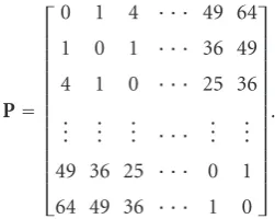
to physically store the first row of the extensor matrix, and each subsequent row can be determined as needed through a sequence of shifts and copies. For the example shown in Figure 1,Imin = 0, Imax = 8,D = 9 and for an intensity
quantization bin size of one,Pis a 9×9 matrix given by
P= ⎡ ⎢ ⎢ ⎢ ⎢ ⎢ ⎢ ⎢ ⎢ ⎢ ⎢ ⎢ ⎢ ⎢ ⎣
0 1 4 · · · 49 64
1 0 1 · · · 36 49
4 1 0 · · · 25 36 ..
. ... ... · · · ... ...
49 36 25 · · · 0 1
64 49 36 · · · 1 0 ⎤ ⎥ ⎥ ⎥ ⎥ ⎥ ⎥ ⎥ ⎥ ⎥ ⎥ ⎥ ⎥ ⎥ ⎦ . (7)
Next, we exploit the redundancy in computing pixel intensity dissimilarities by constructing 1D histograms,hm,n, of each
class from every channel in the image yielding MN his-tograms. The length of each histogram equals the dimension of the extensor matrix P (i.e., D). Histograms have been previously used in level set segmentation, or to speed up
their implementation and is similar to a Chan and Vese style of modeling the image based on some sort of a priori characteristics [2], a fact highlighted at the beginning of this paper.
Thus, for the example shown inFigure 1, histograms for the two regions (i.e.,h1,1forC1, andh1,2forC2) are simply
0 1 2 3 4 5 6 7 8
h1,2
Background 10 9 14 14 4 13 2 2 1
h1,1
Foreground 16 5 6 2 1 1 0 0 0 (8)
Using the permutation matrix and histograms we compute a vector of weights,wm,n, associated with pixels in each class,
and for every channel using the following expression:
wm,n=Phm,n, n∈[1,N], m∈[0,M−1]. (9)
The matrix-vector multiplication associated with (9) is used to update the active contour evolution and is performed at each level set iteration. This is not only a fixed cost operation but can be efficiently computed using Melmans algorithm in (5/4)D2+ O(D) floating point operations for a vector (i.e.,
histogram) of lengthD, instead of the 2D2operations needed
for an arbitrary matrix-vector multiplication [12].
By reducing the 2DM-channel image to a finite number of fixed length 1D histograms, we are able to remove the bottleneck of having toexplicitly compute the dissimilarity matrixWwhich as the authors noted in [1] makes segmenta-tion an untenable operasegmenta-tion, even for relatively small images unless suitable approximations are made. Furthermore, it is easy to observe that using a similar analogy, we can seamlessly extend our approach of computing histograms to segment images in higher dimensionsRn, thus making f-GPAC a competitive alternative to other state-of-the-art segmentation methods.
Thus, computing the homogeneity (i.e., force) terms associated with each region in the original GPAC functional is equivalent to summing up intraclass homogeneity terms from each channel:
fnp= M−1
m=0
Mnpwm,n
Ip,m, andn=1, 2,. . .,N,
(10)
where fn[p] is a vector representing the discrete version of (2) for multichannel data with square brackets indicating array indexing, I[p,m] is the intensity at the pth pixel location in the image from themth channel, and the set of binary masksMn(obtained from a discrete, or crisp version of the Heaviside function) is used to select pixels from the nth region out of theN-classes, for each ofM-channels.
I, a 2D image withM-channels and 2-classes, Input: M, an initial 2D mask (binary)
Scalarsλ1,λ2,μ,τ, and,
An appropriate stopping criterion Output : φ0f, the final 2D mask (binary)
(1) ComputeImin,Imaxfrom allM-channels, andD= Imax − Imin+ 1.
(2) Compute the extensor matrixPand histograms for foreground and background from all Mchannels. (3)Ain,Aout, the foreground and background areas fromM.
(4) Compute a signed Euclidean distance transform (EDT),φk
0, ofMusing any suitable algorithm (cf, [11]).
(5)while(!stopping criterion)do
(6) Compute 1D weighting (of lengthD), using equation (9), for every channelm∈[0,M−1]. (7) /∗Update every pixel in the image∗/
(8) for j=0, 1,. . .,MsNsdo
(9) f1[j]=M−m=01M[j]wm,1[I[j,m]], f2[j]=M−m=01(1−M[j])wm,2[I[j,m]]
(10) Updateφk[j] toφk+1[j] using a semi-explicit discretization of (3) as in [5].
(11) Update maskMand histogramshm,nfor each channel and class, by noting sign changes inφk+1−φk. (12) Update mask M.
(13) UpdateAinandAout.
(14) end for (15)end while
(16) /∗Binary mask from converged level set∗/ (17)φ0f ←M
Algorithm1: Fast GPAC for 2-class image segmentation.
in the two-class (N =2) case, and we use f1and f2 for fin
and fout, respectively (see (1)). For example, even though it
is indicated that two histograms need to be maintained (and updated) for solving the two-class segmentation problem, it is easy to observe that, under certain conditions, this can be reduced to updating a single histogram. Using (10) and (9), and assuming the scaling termsλ1=λ2=λ, we can discretize
and rewrite the data-homogeneity term of (3) as
λ
fout
Aout −
fin
Ain
=λ
M−1
m=0
P
hm,2
Aout −
hm,1
Ain
. (11)
Let us simplify the term within braces. We know that the histogram of the complete image,h = h1,1+h1,2, and the
total area of the imageAΩ = Ain+Aout. On replacingh1,2
andAoutin (11), the terms within the braces can be rewritten
as
λ M−1
m=0
P
hm,2
Aout −
hm,1
Ain
=λ
M−1
m=0
P
h−hm,1
AΩ−Ain −
hm,1
Ain
=λ M−1
m=0
P
Ainh−AΩhm,1
((AΩ−Ain)Ain)
= λin
AΩ
M−1
m=0
Ph
Term 1
− λin
Ain
M−1
m=0
Phm,1,
Term 2
(12)
where
λin= λAΩ
AΩ−Ain.
(13)
Clearly, Term 1 in (12) can be precomputed prior to beginning the iteration process. Hence the performance of f-GPAC can be made entirely dependent on updating a single histogram (Term 2—the histogram of the foreground region). The simplification described above is not valid if kernel-smoothing (e.g., Gaussian, cubic B-splines, etc.) is applied on the histograms prior to computing the homo-geneity terms. However, kernel-smoothing on the image as a preprocessing step is not precluded by this simplification.
3. Experimental Results
We have implemented the proposed f-GPAC algorithm in MATLAB, utilizing calls to dynamic linked libraries written in C++ to optimize for speed. We have compared the performance of our algorithm with the original GPAC algorithm for which source code and test data are available online [13]. Unless otherwise mentioned, the same initial mask, as well as the following parameters, λ1 = NsMs,
λ2 = NsMs, μ = 4.0×10⁴, = 1.0 were used in both
algorithms. In addition, the following tile sizes have been used for the original GPAC algorithm: 4×4, 8×8, and 12 ×12. In the original GPAC implementation, the level set iteration is deemed to have converged if the number of pixels changing signs in two consecutive iterations is less than a certain fixed number [13]. We have also used this stopping condition when implementing our algorithm. A semi-implicit discretization is used to solve the level set update equation (3). We omit details of this discretization and instead direct readers to [5, page 8, Section III].
(a) Fast GPAC—After 0, 3, 6, and 14 iterations
(b) Original GPAC—After 0, 3, 6, and 81 iterations, with tile size of 4×4
(c) Original GPAC—After 0, 3, 6, and 300 iterations, with tile size of 8×8
(d) Original GPAC—After 0, 3, 6, and 300 iterations, with tile size of 12×12
Figure2: Comparative results of using our fast GPAC algorithm vis-`a-vis the original GPAC algorithm in segmenting the “chinese man” image. The RGB image was transformed into the YCbCr space prior to segmentation. It can be noted that decreasing the tile size improves the convergence rate of the level set segmentation (indicated by the white mask). On the other hand, convergence is reached after 14 iterations when using the f-GPAC algorithm. The stopping criterion is satisfied if less than 30 pixels change signs between two successive iterations, or a count of 300 iterations is reached.
perceptual uniform color-space and faster convergence, RGB images were transformed to the YCbCr space and suitably scaled, prior to segmentation. We shift the dynamic range of the image components using the experimentally deter-mined transformation, Y-10, Cb-20, and, Cr-20. We have observed that recentering the color component histograms improves the final image segmentation results. An L2
-squared intensity-based extensor distance matrix (as shown in (5)) of size 256×256 (and storing only the first row, as described inSection 2) was used in all the experiments.
As shown in Figure 2, approximate versions of the original GPAC algorithm lead to a longer convergence time (4×4 tile sizes), or incorrect segmentation (12 ×12 tile sizes). In contrast, our f-GPAC algorithm correctly extracts out the man and similar regions (e.g., Chinese characters) from the image. Using the same parameters, we notice a nearly 7-fold decrease in convergence time when compared to the original GPAC algorithm using the smallest possible tile size dimension. Unfortunately, using the original GPAC algorithm, further reduction in tile size was not possible due to the huge amount of memory needed for storing the dissimilarity matrix. A similar set of observations can be drawn when segmenting other images having similar dimensions (e.g., “horses” and “starfish” inFigure 3).
The f-GPAC algorithm produces nearly the same (or better) results as the original GPAC algorithm, using the smallest computationally feasible tile size for the latter, and f-GPAC also demonstrates faster convergence. Moreover, as observed in [1] increasing tile sizes can lead to unreliable results as seen in Figure 3, where the tile size is increased to 12×12. We wish to emphasize that changing the scaling parameters associated with the level set functional may lead to improved results using the original GPAC method. In our f-GPAC implementation we have avoided this approach and used the same set of parameters for segmenting all images described in the experiments. However, we do acknowledge that even in our algorithm, some parameters may need to be changed (e.g.,μthat controls smoothness of the curve) when segmenting different classes of images.
(a) 0, 3, and 14 iterations (e) 0, 3, and 15 iterations
(b) 0, 3, and 66 iterations, tile size of 4×4 (f) 0, 3, and 104 iterations, tile size of 4×4
(c) 0, 3, and 300 iterations, tile size of 8×8 (g) 0, 3, and 300 iterations, tile size of 8×8
(d) 0, 3, and 300 iterations, tile size of 12×12 (h) 0, 3, and 300 iterations, tile size of 12×12
Figure3: Comparative results at various iteration steps when using our fast GPAC algorithm ((a) and (e)) vis-`a-vis the original GPAC algorithm ((b)–(d), and (f)–(h)) in segmenting “horses” and “starfish” images. The same parameters, used in segmenting the “chinese man” image (Figure 2), were also used in segmenting these images.
(a) f-GPAC-0 iterations (b) f-GPAC-3 iterations (c) f-GPAC-8 iterations (d) f-GPAC-20 iterations
(e) Original GPAC-0 iterations (f) Original GPAC-3 iterations (g) Original GPAC-6 iterations (h) Original GPAC-300 iterations
Figure4: Comparative results of using the f-GPAC algorithm vis-`a-vis the original GPAC algorithm in segmenting “benign cells” with dimensions 557×227. The minimum tile size that could be used in the original GPAC algorithm was 12×12. The stopping condition was set at 60 pixels, or a maximum iteration count of 300. Other parameters (likeλ1,λ2, etc.) were the same as that used in generating results
shown inFigure 3. Evidently, the f-GPAC algorithm correctly segments the background (i.e., noncellular regions), while the original GPAC is only able to segment stromal (white) regions in the image.
hematoxylin and eosin (H&E) stained images of biopsy tissue cores containing various grades of prostrate cancer including, “benign cells” (Figure 4), “grade3 cells” (Figure 5), and “grade4 cells” (Figure 6), respectively. With small tile sizes the original GPAC algorithm cannot be used for segmenting large images (e.g., “grade4 cells”), while using a larger tile size (e.g., 14×14) leads to the eventual disappearance of the evolving curve! However, using the proposed f-GPAC algorithm, a clear demarcation between cellular clusters and the background is achieved in all cases, within 60 iterations. The stopping criterion was changed from 30 to 60 pixels, and the upper bound on the number of iterations set to 300 for this dataset.
(a) f-GPAC-0 iterations (b) f-GPAC-3 iterations (c) f-GPAC-6 iterations (d) f-GPAC-29 iterations
(e) Original GPAC-0 iterations (f) Original GPAC-3 iterations (g) Original GPAC-6 iterations (h) Original GPAC-300 iterations
Figure5: Comparative results of using the f-GPAC algorithm vis-`a-vis the original GPAC algorithm in segmenting “grade3 cells” with dimensions 340×156. The minimum tile size that could be used in the original GPAC algorithm was 5×5. The stopping condition was set at 60 pixels, or a maximum iteration count of 300. Other parameters (likeλ1,λ2, etc.) were the same as those used in generating results shown
inFigure 3. Evidently, both the f-GPAC, as well as the original GPAC algorithm correctly segment the foreground (i.e., cellular regions). However, the large value ofμresults in smoothed blobs when using the original GPAC. Fine details of cell boundaries are preserved when using the f-GPAC algorithm.
(a) f-GPAC-0 iterations (b) f-GPAC-3 iterations (c) f-GPAC-6 iterations (d) f-GPAC-36 iterations
(e) Original GPAC-0 iterations (f) Original GPAC-3 iterations (g) Original GPAC-6 iterations (h) Original GPAC-225 iterations
Figure6: Comparative results of using the f-GPAC algorithm vis-`a-vis the original GPAC algorithm in segmenting “grade4 cells” with dimensions 388×389. The minimum tile size that could be used in the original GPAC algorithm was 14×14. was the same as that used in generating results shown inFigure 5. The selected tile size for the GPAC algorithm leads to the disappearance of the evolving curve. Please refer to the text for more details.
tile size is sufficiently reduced then a correct segmentation is achieved using the original GPAC algorithm (Figure 4). However, there is excessive smoothing of boundaries in the segmented region due to a combination of using image tiling and without tuningμ.
4. Conclusions
with various elements of the complete dissimilarity matrix by fixed length histograms and an intensity-based circulant symmetric-centrosymmetric extensor distance matrix, thus obviating the need to use spatial approximations to the dissimilarity matrix. This dramatically reduces the memory requirement for GPAC as image size increases while still computing exact weights, which inturn leads to faster conver-gence, and accurate segmentation when compared with the original GPAC algorithm. Opportunities for further improv-ing the performance of f-GPAC include usimprov-ing a narrow-band implementation by maintaining a list of narrow-narrow-band pixels around the zero level set and updating only those pixels [9]. This approach is useful when a good initial guess is provided to the f-GPAC algorithm. Parallelization using additive operator splitting (AOS) can also be employed when updating the Euler-Lagrange equation for f-GPAC (cf [21, 22]) to further speed-up performance. The proposed f-GPAC algorithm improves the applicability of GPAC for a wide range of image segmentation tasks and offers scalability to explore automatic segmentation of large multidimensional datasets.
Acknowledgments
The authors would like to thank the U.S. National Institute of Health and the U.S. Department of Defence for financial support that made this research possible. In addition, the authors would like to thank Luca Bertelli and B. S. Manju-nath at the University of California, Santa Barbara for fruitful discussions related to various implementation details of the GPAC algorithm, and Michael Feldman at the University of Pennsylvania, Philadelphia for providing prostrate cancer images used in testing the f-GPAC algorithm. This work was initiated at the University of Missouri-Columbia under a U.S. National Institute of Health NIBIB award R33 EB00573 and completed at Rensselaer Polytechnic Institute, Troy with kind support from Dr. Badrinath Roysam under a U.S. DOD Cancer Research Program IDEA Grant BC061142.
References
[1] B. Sumengen and B. Manjunath, “Graph partitioning active contours (GPAC) for image segmentation,”IEEE Transactions on Pattern Analysis and Machine Intelligence, vol. 28, no. 4, pp. 509–521, 2006.
[2] T. Brox and J. Weickert, “Level set based image segmentation with multiple regions,” in Proceedings of the 26th Pattern Recognition Symposium (DAGM ’04), vol. 3175 ofLecture Notes in Computer Science, pp. 415–423, Tubingen, Germany, August 2004.
[3] F. Bunyak, K. Palaniappan, S. Nath, and G. Seetharaman, “Flux tensor constrained geodesic active contours with sensor fusion for persistent object tracking,”Journal of Multimedia, vol. 2, no. 4, pp. 20–33, 2007.
[4] Y. Boykov, O. Veksler, and R. Zabih, “Fast approximate energy minimization via graph cuts,” IEEE Transactions on Pattern Analysis and Machine Intelligence, vol. 23, no. 11, pp. 1222– 1239, 2001.
[5] T. Chan and L. Vese, “Active contours without edges,” Tech. Rep. CAM98-53, Department of Mathematics, UCLA,
Los Angeles, Calif, USA, December 1998,ftp://ftp.math.ucla .edu/pub/camreport/cam98-53.ps.gz.
[6] L. Bertelli, B. Sumengen, B. S. Manjunath, and F. Gibou, “A variational framework for multi-region pairwise similarity-based image segmentation,” IEEE Transactions on Pattern Analysis and Machine Intelligence, vol. 30, no. 8, pp. 1400– 1414, 2008.
[7] L. A. Vese and T. F. Chan, “A multiphase level set framework for image segmentation using the Mumford and Shah model,”
International Journal of Computer Vision, vol. 50, no. 3, pp. 271–293, 2002.
[8] A. Hafiane, F. Bunyak, and K. Palaniappan, “Clustering initiated multiphase active contours and robust separation of nuclei groups for tissue segmentation,” inProceedings of the 19th International Conference on Pattern Recognition (ICPR ’08), pp. 1–4, Tampa, Fla, USA, December 2008.
[9] S. Nath, K. Palaniappan, and F. Bunyak, “Cell segmentation using coupled level sets and graph-vertex coloring,” in Pro-ceedings of the 9th International Conference on Medical Image Computing and Computer-Assisted Intervention (MICCAI ’06), vol. 4190 ofLecture Notes in Computer Science, pp. 101–108, Springer, Copenhagen, Denmark, October 2006.
[10] K. Palaniappan, J. Uhlmann, and D. Li, “Extensor-based image interpolation,” inProceedings of IEEE International Conference on Image Processing (ICIP ’03), vol. 2, pp. 945–948, Barcelona, Spain, September 2003.
[11] P. Felzenswalb and D. Huttenlocher, “Distance transforms of sampled functions,” Tech. Rep. TR2004-1963, Department of Computer Science, Cornell University, Ithaca, NY, USA, September 2004, http://people.cs.uchicago.edu/∼pff/papers/ dt.pdf.
[12] A. Melman, “Symmetric centrosymmetric matrix-vector mul-tiplication,”Linear Algebra and Its Applications, vol. 320, no. 1–3, pp. 193–198, 2000.
[13] http://vision.ece.ucsb.edu/∼lbertelli/soft GPAC.html. [14] A. Mosig, S. J¨aeger, W. Chaofeng, et al., “Tracking cells in live
cell imaging videos using topological alignments,”Algorithms for Molecular Biology, vol. 4, article 10, pp. 1–9, 2009. [15] S. K. Nath, F. Bunyak, and K. Palaniappan, “Robust tracking
of migrating cells using four-color level set segmentation,” in
Proceedings of the 8th International Conference on Advanced Concepts for Intelligent Vision Systems (ACIVS ’06), vol. 4179 ofLecture Notes in Computer Science, pp. 920–932, Antwerp, Belgium, September 2006.
[16] F. Bunyak, K. Palaniappan, S. K. Nath, T. I. Baskin, and D. Gang, “Quantitative cell motility for in vitro wound healing using level set-based active contour tracking,” inProceedings of the 3rd IEEE International Symposium on Biomedical Imaging (ISBI ’06), pp. 1040–1043, Arlington, Va, USA, April 2006. [17] G. Dong, T. I. Baskin, and K. Palaniappan, “Motion flow
esti-mation from image sequences with applications to biological growth and motility,” inProceedings of the IEEE International Conference on Image Processing (ICIP ’06), pp. 1245–1248, Atlanta, Ga, USA, October 2006.
[18] C. M. van der Weele, H. S. Jiang, K. K. Palaniappan, V. B. Ivanov, K. Palaniappan, and T. I. Baskin, “A new algorithm for computational image analysis of deformable motion at high spatial and temporal resolution applied to root growth. Roughly uniform elongation in the meristem and also, after an abrupt acceleration, in the elongation zone,”Plant Physiology, vol. 132, no. 3, pp. 1138–1148, 2003.
Workshop (CVPRW ’04), pp. 25–33, IEEE Computer Society, Washington, DC, USA, June-July 2004.
[20] A. Hafiane, F. Bunyak, and K. Palaniappan, “Fuzzy clustering and active contours for histopathology image segmentation and nuclei detection,” inProceedings of the 10th International Conference on Advanced Concepts for Intelligent Vision Systems (ACIVS ’08), vol. 5259 ofLecture Notes in Computer Science, pp. 903–914, Springer, Juan-les-Pins, France, October 2008. [21] J. Weickert, B. M. Ter Haar Romeny, and M. A. Viergever, “Effi
-cient and reliable schemes for nonlinear diffusion filtering,”
IEEE Transactions on Image Processing, vol. 7, no. 3, pp. 398– 410, 1998.