Implementation of computation-reduced DCT using a novel method

(1)

R E S E A R C H

Open Access

Implementation of computation-reduced

DCT using a novel method

K. K. Senthilkumar

1

, K. Kunaraj

2*

and R. Seshasayanan

1

Abstract

The discrete cosine transform (DCT) performs a very important role in the application of lossy compression for representing the pixel values of an image using lesser number of coefficients. Recently, many algorithms have been devised to compute DCT. In the initial stage of image compression, the image is generally subdivided into smaller subblocks, and these subblocks are converted into DCT coefficients. In this paper, we present a novel DCT architecture that reduces the power consumption by decreasing the computational complexity based on the correlation between two successive rows. The unwanted forward DCT computations in each 8 × 8 sub-image are eliminated, thereby making a significant reduction of forward DCT computation for the whole image. This algorithm is verified with various high- and less-correlated images, and the result shows that image quality is not much affected when only the most significant 4 bits per pixel are considered for row comparison. The proposed architecture is synthesized using Cadence SoC Encounter® with TSMC 180 nm standard cell library. This architecture consumes 1.257 mW power instead of 8.027 mW when the pixels of two rows have very less difference. The experimental result shows that the proposed DCT architecture reduces the average power consumption by 50.02 % and the total processing time by 61.4 % for high-correlated images. For less-correlated images, the reduction in power consumption and the total processing time is 23.63 and 35 %, respectively.

Keywords:DCT, IDCT, Image compression, FPGA, ASIC

1 Introduction

Image compression is a process of reducing the size of representation of graphics file in binary format without affecting the quality of the image to an objectionable level. This reduction helps to store more images for the same amount of storage device. It also decreases the transmission time for images to be sent over the various technologies like internet [1]. The discrete cosine transform (DCT) which is the most widely used technique for image compres-sion was initially defined in [1]. It came up as a revolutionary standard when compared with the other existing transforms. After that, an algorithm for computing Fast DCT (FDCT) was introduced by Chen et al., in [2] which was based on matrix decom-position of the orthogonal basis function of the cosine transform. This method took (3N/2)(log2N−1) + 2 real

additions andNlog2N−3 N/2+ 4 real multiplications, and this is approximately six times faster than the conventional approach. Further, a new algorithm was introduced for the 2Npoint DCT as in [3]. This algorithm uses only half of the number of multiplications required by the existing efficient algorithms (12 multiplications and 29 additions), and it makes the system simpler by decom-posing the N-point Inverse DCT (IDCT) into the sum of two N/2-point IDCTs. A recursive algorithm for DCT [4] was presented with a structure that allows the generation of the next higher order DCT from two identical lower order DCTs to reduce the number of ad-ders and multipliers (12 multiplications and 29 additions). Loffler came up with a practical fast 1-D DCT algorithm [5] in which the number of multiplications was reduced to 11 by inverting add/subtract modules and found an equivalence for the rotation block (only 3 additions and 3 multiplications per block instead of 4 multiplications and 2 additions). Following these contributions in DCT imple-mentation, many algorithms were constantly introduced to optimize the DCT.

* Correspondence:[email protected]

2_{Department of ECE, Loyola-ICAM college of Engineering and Technology} (LICET), Chennai 600034, India

Full list of author information is available at the end of the article

(2)

In recent years, the idea of implementing DCT using CORDIC (co-ordinate rotation digital computer) [6] using only shift and add arithmetic with look-up tables was ana-lyzed for efficient hardware implementation. Another tech-nique called distributed arithmetic (DA) was devised [7] which computes multiplication as distributed over bit-level memories and adders. Read-only memory (ROM) free 1-D DCT architecture was discussed in [8], and this architecture is based on DA method with reduced area and power re-duction. As in [9], an unsigned constant coefficient multi-plication was done by moving two negative signs to the next adder to make them positive, and it was imple-mented using multiplier-less operation. The prime N-length DCT was divided into similar cyclic convolution structures, and the DCT was implemented using sys-tolic array structure [10]. The technique used in [11] re-duced the resource usage and increased the maximum frequency by rearranging the ADD blocks to the consecu-tive stages. Also, to eliminate the use of multipliers by using shift and addition operations, many algorithms were devised. The technique which uses Ramanujan numbers for calculating cosine values and uses Chebyshev type re-cursion to compute DCT [12] was also proposed. A low power multiplier-less DCT was presented in [13], and it re-duces the switching power consumption around 26 % by removing unnecessary arithmetic operations on unused bits during the CORDlC calculations. The complexity of DCT computation was reduced in [14] by optimizing the Loeffler DCT, based on the CORDlC algorithm. Further, it reduces the 11 multiply and 29 add operations to 38 add and 16 shift operations without losing quality. A low power design technique was presented in [15], which eliminates DCT computation of low energy macro block. A technique was presented to reduce the complexity of multiplications in DCT [16] by using differential pixels in 8 × 8 blocks of input image matrix. Based on differences of 64 DCT coeffi-cients, separate operand bit-widths were used for different frequency components to reduce computation energy [17]. Various low-power design techniques such as dual voltage, dual frequency, and clock gating were used in the DCT architecture to reduce the power consumption [18].

This paper proposes a new architecture that com-putes the DCT, based on the difference between pixels of two rows, and also, it reduces the computations and power consumption of DCT. The paper is organized as follows: The most common DCT implementation strategies are discussed in Section 2. The conventional

image compression technique using DCT and the pro-posed comparative input method (CIM) which elimi-nates the unwanted DCT computations are discussed in Section 3. The simulation results, performance, and comparative analysis of the proposed DCT is given in Section 4, and Section 5 concludes the research findings.

2 Existing algorithms for DCT implementation Generally, the two methods used for computing 2-D DCT are

(i) Direct 2-D computation and

(ii)Decomposition into two 1-D DCTs using seperability.

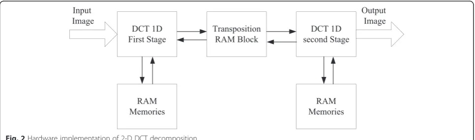
The proposed method adopts the second approach to compute the 2-D DCT. The row transformation is initially applied to obtain a 1-D output and then applying it the next time along the column yields the 2-D output as shown in Fig. 1. In hardware imple-mentation of 2-D DCT, the inputs can be obtained by storing them in random access memory (RAM), and then, it is given to the 1-D computation module. After the computation, the output is stored in a transposition buffer before it is given to the 1-D block again. This is illustrated in Fig. 2.

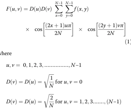
The 2-D DCT is given by Eq. (1).

F uð ;vÞ ¼D uð ÞD vð Þ X

N−1

x¼0

X

N−1

y¼0 f xð ;yÞ

cos ð2xþ1Þuπ 2N

cos ð2yþ1Þvπ 2N

ð1Þ

where

u;v¼ 0;1;2;3;………;N−1

D vð Þ ¼D uð Þ ¼

ffiffiffiffi

1 N

r

foru;v¼0

D vð Þ ¼D uð Þ ¼

ffiffiffiffi

2 N

r

foru;v¼1;2;3……:;ðN−1Þ

In the Eq. (1), f(x,y) is the input matrix of pixels representing the N×N sub-image. F(u,v) is the

(3)

corresponding 2-D DCT output coefficients. D(u) and

D(v) are the normalizing factors. Both the cosine terms represent the orthonormal basis functions of the cosine functions used to map the input pixels into the transformed coefficients. The input values should be multiplied with the orthonormal basis func-tions and the normalizing factor to get the DCTcoef-ficients. The 1-D DCT is given in the Eq. (2).

F uð Þ ¼D uð Þ X

N−1

x¼0

f xð Þ cos ð2xþ1Þuπ 2N

ð2Þ

for

u¼0;1;2…N−1

D uð Þ ¼

ffiffiffiffi

1 N

r

foru¼0

D uð Þ ¼

ffiffiffiffi

2 N

r

foru¼1;2;3……:;ðN−1Þ

Here, f(x) is the 1-D row of input pixels, and the co-sine term is the orthonormal basis function. F(u) is the 1-D DCT output, andD(u) is the normalizing factor.

To implement the DCT, modified Lee’s algorithm [3] and Chen’s algorithm [2] are used in this paper. Lee’s al-gorithm utilizes three levels of mathematical decompos-ition to calculate DCT in a simpler method. Compared to Chen’s algorithm, Lee’s method reduces the computa-tional complexity of calculating DCT coefficients by 46 %. Both the algorithms are simulated using Matlab and EDA tool. To prove the hardware efficiency of the proposed algorithm, the architecture is implemented in field programmable gate array (FPGA). The design entry is made through Verilog hardware description language (HDL), simulated in Xilinx ISim, and synthesized using Xilinx XST.

2.1 Fast algorithm

The algorithm proposed by Chen et al. [2] to compute forward DCT is called “Fast algorithm.” The computa-tion is done similar to the method shown in Fig. 2 by computing 1-D DCT, transposing it, and then comput-ing 2-D DCT. For a 2-D DCT, the 8 × 8 transformation matrix corresponding to the 8 × 8 basis function is given by A¼ d d a c d d e g d d −g −e

d d −c −a b f

c −g

−f −b −a −e

−b −f e a

f b g −c d −d

e −a −d d

g c

d −d −c −g

−d d a −e f −b

g −e b −f c −a

−f b a −c

−b f e −g

2 6 6 6 6 6 6 6 6 6 4 3 7 7 7 7 7 7 7 7 7 5

whereb¼C1;c¼C2;d¼C3;a¼C4;e ¼C5;f ¼C6;g¼C7;

Ci¼0:5 cosðiπ=16Þ

In Chen’s algorithm, the 8 × 8 transformation matrix is decomposed into two 4 × 4 matrices. This is done by con-sidering the input values which should be multiplied with common coefficients (in the transformation matrix). After decomposing the 8 × 8 transformation matrix, the two 4 × 4 transformation matrices obtained are

Yð Þ0 Yð Þ2 Yð Þ4 Yð Þ6

0 B B @ 1 C C A¼ a c a f a f −a −c a −f −a c a −c a −f 0 B B @ 1 C C A

Xð Þ þ0 Xð Þ7 Xð Þ þ1 Xð Þ6 Xð Þ þ2 Xð Þ5 Xð Þ þ3 Xð Þ4

0 B B @ 1 C C A

Yð Þ1 Yð Þ3 Yð Þ5 Yð Þ7

0 B B @ 1 C C A¼ b d e g d −g −b −e e −b g d g −e d −b 0 B B @ 1 C C A

Xð Þ0 −Xð Þ7 Xð Þ1 −Xð Þ6 Xð Þ2 −Xð Þ5 Xð Þ3 −Xð Þ4

0 B B @ 1 C C A

(4)

computations involved is (3N/2)(log2N−1) + 2 additions and Nlog2N−3N/2 + 4 multiplications. Hence, forN= 8, it requires 16 multiplications and 12 additions.

3 Image compression using DCT

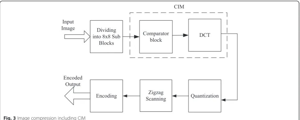
The overall image compression using the proposed CIM is carried out by performing the steps shown in Fig. 3. Initially, the input image is subdivided into smaller sub-images of size 2n, so that the correlation (redundancy) between the adjacent pixels in the sub-image will reduce the number of DCT coefficients. In general, both the level of computational complexity and compression in-creases as the sub-image size inin-creases. The most popu-lar sub-image sizes are 8 × 8 and 16 × 16, and we consider sub-image size of 8 × 8 to have optimal compu-tational complexity. Also, the frequency transformations like DCT are good at compressing smooth areas with low frequency content, but quite bad at compressing high frequency contents.

After performing CIM-based DCT computation, the following steps for the compression of the image are carried out. The DCT coefficients are quantized to a pre-determined level to reduce psycho-visual redundancy. Zigzag scanning ensures the scanning of high-frequency DCT coefficients, and the scanned coefficients are encoded to reduce coding redundancy.

3.1 DCT computation through CIM

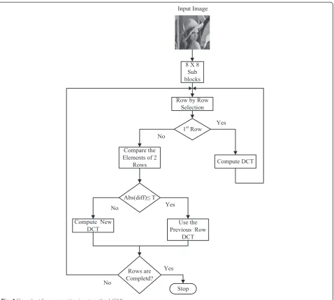
The comparative input method is a new approach of com-paring two adjacent rows in anN×Nsub-image while cal-culating the forward 1-D DCT. Initially, the 8 × 8 block of the sub-images are obtained through subdivision process. In general, every row of the sub-image (an array of eight

elements) is applied as input to the 1-D DCT to obtain an output array of eight DCT coefficients.

For a considered sub-image, the DCT is computed for the first row. From the second row onwards, pixels in each row are compared with the previous row of pixels. If all the pixels of a row is found to be nearly same as the pixels in the previous row, the DCT computation need not be performed for the second row. Instead, the previous row’s 1-D DCT coefficients can be used for the current second row without any need for computation. Otherwise, the pixels are considered as non-matching and the comparison fails. For this case, 1-D DCT is ap-plied again for the particular row to obtain a new DCT coefficients. This procedure is applied for all the remaining rows of the 8 × 8 sub-image. By following this row comparison, a large number of computations are eliminated. Figure 4 shows the above discussed comparison method for DCT computation.

Consider Xm is the mth row of the given image,

Xm(n) is the nth pixel corresponding to the mth row of the original image. Similarly,Ymis the DCT output for mth row of the image,Ym(n) is the nth DCT coefficient corresponding to the mth row. Thus, the DCT coeffi-cient is computed as follows:

Ym ¼ Ym‐1; if abs ðXmð Þn ‐ Xm‐1ð ÞnÞ≤T ;

forn¼1; 2…8 ¼ Ym; otherwise

ð3Þ

Here, the threshold value depends on the number of bits considered for row comparison. If the absolute dif-ference between any of the pixels inXmandXm-1is less than or equal to the given threshold (T) value, it is

(5)

considered as matching otherwise it is assumed to be non-matching. With these assumptions, the Eq. (3) is used to eliminate the DCT computation (Ym) for that particular row, if the row (Xm) is matched with previous row (Xm-1). Based on the required image quality while reconstruction, the threshold value is selected as 1 or 3 or 7 or 15 for efficient hardware implementation. Choos-ing higher threshold value slightly reduces the image quality while reconstruction.

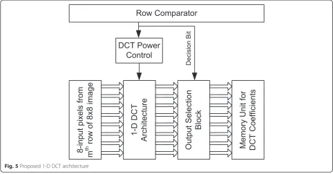
3.2 Proposed DCT architecture using CIM

The proposed 1-D DCT architecture is implemented using CIM to perform the forward DCT, and it is shown

in Fig. 5. The main components of the proposed system are

1. Row-comparator 2. DCT power controller 3. DCT computation unit 4. Output selection block 5. Memory

(6)

or deactivates the DCT core. Thus, the main function of the DCT power control block is to control the power input given to the DCT architecture. If it receives a

“high”signal, it disables the power to be supplied to the DCT architecture else it enables the power input. Hence, if the two rows of an 8 × 8 sub-image are equal, the DCT need not be computed for the current row, and thus, significant power reduction is achieved. Also, the output selection block provides the buffered pre-computed DCT coefficients of the previous row or the output of the DCT core of the current row based on the input provided by the row comparator. Finally, the DCT coefficients of the 8 × 8 sub-image are stored in a RAM for further processing.

3.3 Average power consumption (Pav)

ConsiderPαas the average power consumption of DCT without the row comparison unit andPβas the average power consumption of all the other units excluding DCT core which is used for comparing rows. Ncom is the total number of 8 × 1 rows available in the image.

Nrepis the number of rows of 8 × 1 pixels having similar pixel values and excluding the first row; Nnon-repis the number of rows of 8 × 1 pixels having dissimilar pixel values, and also, it includes first row having similar pixel values.Pavis the average power consumed by the proposed DCT architecture and is given by Eq. (4). The Eq. (5) provides the percentage of power reduction that is obtained using proposed DCT architecture when compared with the regular DCT implementation.

Pav ¼ PαNnon repþPβNcom

=Ncom ð4Þ

% power reduction¼ð1Pav=PαÞ 100 ð5Þ

3.4 Processing time (Tpr)

ConsiderT_αas the time required to process a 1-D DCT for a single row andT_βas the time required to process a 1-D DCT for a single row when the current row matches with previous row. Ncom is the number of 1-D computations involved in an image,Nrepis the number of 1-D computations repeated, Nnon-rep is the number of non-repeated 1-D computation, and Ttot is the total time required to process the 1-D DCT for an image by the proposed DCT architecture, and it is given by Eq. (6). The Eq. (7) shows the percentage processing time (Tpr) reduction using proposed DCT architecture com-paring with regular DCT implementation.

Ttotal ¼TαNnon comþTβNcom ð6Þ

% processing timeðTPRÞ reduction ¼ 1 Ttot

TαNcom

ð Þ

100 ð7Þ

4 Results and discussions

(7)

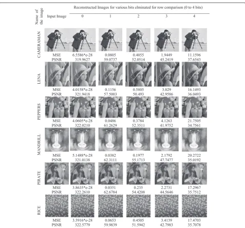
metrics like mean squared error (MSE) and peak signal to noise ratio (PSNR) are calculated. Figure 6 shows the reconstructed images simulated using Matlab and the MSE; PSNR values are also listed for each image. The experiment is conducted for differ-ent cases of various thresholds based on the number of MSBs considered for row comparison.

Different images with wide variations in the intensity are considered for computing DCT using the proposed method. Performance comparison for various images obtained from the proposed DCT computation is given in Fig. 6 along with the output images. From Fig. 6, it is clear that the output image is exactly same as the

input image when 0 bit is ignoredfor row comparison. When the number of bits ignored per pixel increases, the image quality decreases slightly. The comparison of MSE and PSNR values obtained for each case of dif-ferent input images are given in Table 1. For all the output images, the MSE value increases when the number of bits per pixel ignored for row comparison increases and makes the PSNR to decrease.

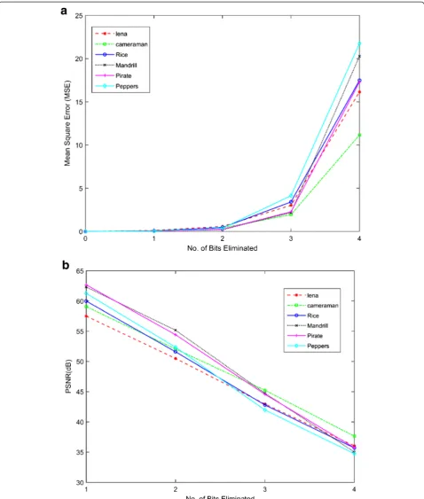
A plot between the MSE values and the number of bits ignored per pixel corresponding to various images is depicted in Fig. 7a. The MSE values are less till the number of bits ignored per pixel is less than 3. When 3 bits are ignored, the MSE is considerable and if the

(8)

number of bits ignored becomes 4, the MSE value be-comes significantly high. This is because in the latter case, the difference between the two pixels (for row comparison) becomes 15 which causes a significant difference in the DCT coefficient.

Figure 7b shows the corresponding PSNR of the reconstructed images as given in Table 1. The chart shows a degradation in the image quality as the num-ber of bits ignored for row comparison increases. When the comparison is made between the various in-puts, it can be seen that the PSNR for the Cameraman image is high, compared with the other images for 4-bit eliminationand hence a better output quality.

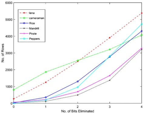
To calculate the reduction in the computational com-plexity, we have found the number of repeated rows for which DCT needs not be calculated. The repeated number of rows for various number of elminated bit for row comparison is shown in Table 2.

Figure 8 plots the number of repeated rows as given in Table 2. Based on the homogeneity of pixels in the sub-images, the interpixel redundancy varies, and hence, the number of repeated rows changes for each image.

4.1 FPGA implementation of DCT using CIM

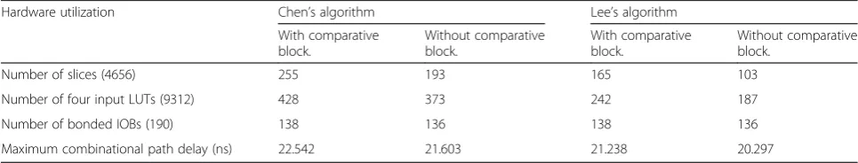
FPGA consists of large number of configurable logic blocks (CLBs) connected together through connection matrix to form any complicated high speed digital sys-tems. FPGA implementation is a suitable solution for testing the performance of the proposed architecture before the development of ASIC. All the hardware sub-blocks of the design is developed with the Verilog HDL and verified with the Xilinx ISim simulator. Figure 9 shows the simulation results of DCT using ISim, and these results are verified with the results obtained usingMatlab. After the functional verification, the de-sign is synthesized using Xilinx XST with the Spartan 3e FPGA (3s500eft256-4) as the target device. Table 3 shows the device utilization summary for both the Chen’s and Lee’s algorithm with and without compara-tive blocks.

The input image is converted into its equivalent bin-ary value using Matlab, and it is given as input to the proposed algorithm implemented using HDL. Using XILINX ISim simulator, the simulation is performed and the corresponding output is stored in a file for further processing. The stored output file is converted into image using Matlab, to calculate image quality metrics like MSE and PSNR. Table 4 shows the MSE and the PSNR values of the reconstructed image from the DCT coefficients computed by simulating the HDL design in XILINX ISim.

Figure 10 plots the MSE of the reconstructed image from the DCT coefficients calculated by simulating the algorithm in XILINX ISim simulator. The simulation is performed by truncating the least significant bits (LSB) of sizes ranging from 1 to 4 (N= 1 to 4) for row comparison. As N is increased from 1 to 4, the com-putational complexity reduces and the MSE increases as shown in Fig. 10. There is a small variation in the MSE and PSNR values obtained from hardware and software implementations.

Figure 11 shows the PSNR of the reconstructed image from the DCT coefficients obtained by simulating the algorithm in XILINX ISim simulator. The PSNR of the reconstructed image reduces as the number of bits for row comparison,Nis increased.

The FPGA hardware resource utilization and the maximum combinational path delay of two DCT archi-tectures are shown in Fig. 12a, b, respectively. From the device utilization summary, 32.25 % of FPGA hard-ware resource is utilized additionally, as the CIM block is included. But, the CIM block eliminates a maximum of 65 % DCT computations for Cameraman image and 39 % reduction for mandrill image.

4.2 ASIC implementation of proposed DCT

The proposed DCT architecture with Lee’s algorithm is synthesized using Cadence SoC Encounter® with TSMC 180 nm library. Table 5 provides the gate count and the power consumption for regular and proposed DCT architecturewith CIM block.

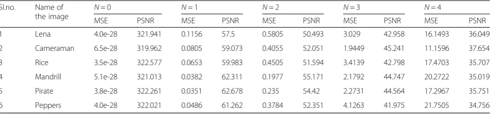
Table 1Comparison of MSE and PSNR of the reconstructed images for different number of bits (N) ignored for row comparison

Sl.no. Name of the image

N= 0 N= 1 N= 2 N= 3 N= 4

MSE PSNR MSE PSNR MSE PSNR MSE PSNR MSE PSNR

1 Lena 4.0e-28 321.941 0.1156 57.5 0.5805 50.493 3.029 42.958 16.1493 36.049

2 Cameraman 6.5e-28 319.962 0.0805 59.073 0.4055 52.051 1.9449 45.241 11.1596 37.654

3 Rice 3.5e-28 322.577 0.0653 59.983 0.4505 51.594 3.4139 42.798 17.4703 35.707

4 Mandrill 5.1e-28 321.013 0.0382 62.311 0.1977 55.171 2.1792 44.747 20.2722 35.019

5 Pirate 3.8e-28 322.261 0.0351 62.678 0.235 54.42 2.2731 44.564 17.2967 35.751

(9)

(10)

The proposed DCT core consumes more cell area as given in Table 5 due to the additional CIM block for reducing the overall computational complexity. When two rows are termed similar, DCT coefficients need not be computed for the later row, and the DCT

coefficients of the previous row can be used. This eliminates the need to use the DCT core, and only the CIM block is active. Hence, using this proposed method, 1251 gates are idle and the DCT is computed with 1.257 mW instead of 8.0157 mW power

Fig. 8Number of rows repeated for various images afterNnumber of bits are ignored for row comparison

Table 2Number of rows repeated for various images afterNnumber of bits are ignored for row comparison

Image N= 0 N= 1 N= 2 N= 3 N= 4

Lena 268 1255 2496 3911 5382

Cameraman 809 1868 2556 3213 4077

Rice 34 357 1304 2774 4310

Mandrill 21 122 495 1374 3220

Pirate 62 224 693 1653 3292

(11)

consumption as the DCT core is disabled. Table 6 compares the power consumption of the regular DCT, the proposed DCT architecture. In Table 6, the power consumption for ignoring 0, 1, 2, 3, and 4 bits are cal-culated using the formula given in Eq. (4), and the per-centage power variations are calculated using Eq. (5).

If all the bits are considered for comparing two pixel values, the proposed DCT power consumption (the average power (pav)) is higher than the normal DCT power consumption (pα) while computing DCT of a sub-image. The power consumed by the comparison unit is greater than the power saved by row elimination in total for the complete image while all the bits are considered. Hence, the percentage power reduction are negative. Whereas in case of ignoring 1 bit for compri-son, the power consumption for the proposed DCT is

higher than that for normal DCT for all the images ex-cept the Cameraman image since it has a great reduc-tions in the number of repeated rows (1868). Hence, the percentage power variations are positive for that image alone. Even in case of ignoring 2 bits, the power reduction may be achieved and it depends on the number of repeated row in an image. Perhaps, by ig-noring 3 or 4 bits for row comparison, significant power reduction can be achieved, and it is clear from the values given in Table 6.

The Fig. 13 plots the percentage power reduction for various images corresponding to various number of bits eliminated for row comparison to avoid the DCT computation.

If two rows matches in pixel value, the DCT coeffi-cients need not be computed and the DCT coefficoeffi-cients Fig. 9Simulation result for 1-D DCT

Table 3Device utilization and timing summary of DCT architecture with and without comparison block

Hardware utilization Chen’s algorithm Lee’s algorithm

With comparative block.

Without comparative block.

With comparative block.

Without comparative block.

Number of slices (4656) 255 193 165 103

Number of four input LUTs (9312) 428 373 242 187

Number of bonded IOBs (190) 138 136 138 136

(12)

of the previous row can be retained. This eliminates the latency in computing DCT for the current row. Based on the correlation between the rows, the overall computational time can be greatly eliminated. If the DCT core is disabled, the overall time consumption to calculate DCT coefficients for a single pixel row is

equal to the latency introduced by the comparator block. The power reduction is achieved by disabling the DCT core power supply when the two row values are same. This can be done using simple buffer and in-verter circuit as shown in Fig. 14. The sizing of the CMOS [22] inverter which controls the power input to Table 4MSE and PSNR of the reconstructed images for various number of bits (N) ignored for row comparison

Sl. no.

Name of the image

N= 0 N= 1 N= 2 N= 3 N= 4

MSE PSNR (dB) MSE PSNR (dB) MSE PSNR (dB) MSE PSNR (dB) MSE PSNR (dB)

1 Lena 0.0004 82.003 0.131 56.951 0.651 49.997 3.672 42.482 18.645 35.425

2 Cameraman 0.0005 80.888 0.090 58.613 0.453 51.568 2.259 44.592 12.870 37.035

3 Rice 0.0002 86.370 0.072 59.539 0.495 51.184 3.765 42.374 19.689 35.189

4 Mandrill 0.0009 78.400 0.043 61.837 0.224 54.632 2.491 44.167 23.358 34.446

5 Pirate 0.0002 84.707 0.039 62.265 0.268 53.848 2.567 44.036 19.779 35.169

6 Peppers 0.0004 82.568 0.054 60.791 0.418 51.921 4.596 41.507 25.046 34.143

(13)

the DCT core is based on the power consumed by the DCT core and its input capacitance which depends on the technology.

The Table 7 shows the comparison of the regular DCT processing time and the proposed DCT architecture pro-cessing time. In the Table 7, the propro-cessing time for ig-noring 0, 1, 2, 3, and 4 bits are calculated using the formula given in Eq. (6) and the percentage processing time reduction is calculated as given in Eq. (7).

Table 8 provides the maximum PSNR achieved and maximum power reduction while reconstructing Lena image from its DCT coefficient. Also, it compares the PSNR and power reduction (%) of various techniques available in the literature for the same image. The pro-posed method reduces the power by 50 % compared to other methods while achieving a maximum PSNR of 35.425 dB for Lena image.

5 Conclusions

(14)

a

b

Fig. 12aFPGA area utilization of the proposed DCT implementation.bMaximum combinational path delay of the proposed DCT implementation

Table 5Comparison of gate count and power consumption

Description DCT architecture

(Lee’s algorithm)

DCT with proposed row comparison unit

Gate counts 1251 1656

Cell area (μm2) 35992 57829

(15)

Table 6Power reduction in the proposed DCT for various number of bits (N) ignored for row comparison

Image Power consumption N= 0 N = 1 N= 2 N= 3 N= 4

Comparison unit power consumption (mW)

Power consumed by DCT alone (mW)

Proposed DCT power consumption (mW)

Power variations in %

Lena 1.26 8.02 9.01 −12.4 8.04 −0.4 6.83 14.8 5.45 32.1 4.01 50.0

Camera 1.26 8.02 8.48 −5.8 7.44 7.1 6.77 15.5 6.13 23.5 5.28 34.1

Rice 1.26 8.02 9.24 −15.3 8.92 −11.3 8 0.2 6.56 18.2 5.06 36.9

Mandrill 1.26 8.02 9.25 −15.4 9.15 −14.2 8.79 −9.6 7.93 1.1 6.12 23.6

Pirate 1.26 8.02 9.21 −14.9 9.05 −12.9 8.59 −7.2 7.65 4.5 6.05 24.5

Peppers 1.26 8.02 9.26 −15.6 9.08 −13.3 8.33 −3.9 6.52 18.6 4.65 42.0

r

et

al.

EURASIP

Journal

on

Image

and

Video

Process

ing

(2015) 2015:34

Page

15

of

(16)

Fig. 13Percentage reduction in power consumption of various images whenNnumber of bits are eliminated (N= 0, 1, 2…4)

(17)

Table 7Reduction in the processing time of proposed DCT architecture for various number of bits (N) ignored for row comparison

Name of image

Processing time of comparison unit (ns)

Processing time of DCT alone (ns)

N = 0 N = 1 N = 2 N = 3 N = 4

Total processing time of proposed design (μs)

% processing time reduction

Lena 0.9 21.6 178.9 −1.0 157.6 11.0 130.7 26.1 100.2 43.4 68.4 61.4

Cameraman 0.9 21.6 167.2 6.0 144.3 18.0 129.5 26.9 115.3 34.9 96.6 45.4

Rice 0.9 21.6 183.9 −4.0 177.0 0.0 156.5 11.6 124.7 29.5 91.6 48.3

Mandrill 0.9 21.6 184.2 −4.0 182.0 −3.0 174.0 1.7 155.0 12.4 115.1 35.0

Pirate 0.9 21.6 183.3 −4.0 179.8 −2.0 169.7 4.1 149.0 15.8 113.6 35.8

Peppers 0.9 21.6 184.5 −4.0 180.4 −2.0 163.8 7.4 123.9 30.0 82.5 53.4

r

et

al.

EURASIP

Journal

on

Image

and

Video

Process

ing

(2015) 2015:34

Page

17

of

(18)

power instead of 8.027 mW with 24.4 % of additional hardware cost when the pixels of two rows have very less difference. The experimental result shows that the power consumption proposed DCT architecture is reduced to 4.01 mW for highly uncorrelated images and 6.02 mW for less-correlated images without much affecting the image quality. This achieves maximum power reduction of 50.02 % and minimum power reduction of 23.63 % of original DCT implementation.

Competing interests

The authors declare that they have no competing interests.

Author details

1

Department of ECE, CEG, Anna University, Chennai 600025, India. 2_{Department of ECE, Loyola-ICAM college of Engineering and Technology} (LICET), Chennai 600034, India.

Received: 6 January 2015 Accepted: 20 October 2015

References

1. N. Ahmed, T. Natarjan, K.R. Rao, Discrete cosine transform. IEEE T Comput 23(2), 90–93 (1974)

2. W.H. Chen, C.H. Smith, S.C. Fralick, A fast computational algorithm for the discrete cosine transform. IEEE T Commun25(9), 1004–1009 (1977) 3. B. Lee, A new algorithm to compute the discrete cosine transform. IEEE T

Acoust Speech P32(6), 1243–1245 (1984)

4. H.S. Hou, A fast recursive algorithm for computing the discrete cosine transform. IEEE T Acoust Speech35(10), 1455–1461 (1987)

5. C. Loeffler, A. Lightenberg, G.S. Moschytz, Practical fast 1–D DCT algorithms with 11 multiplications. Proc Int Conf Acoust Speech Signal Process2, 988–991 (1989)

6. J. Rohit Kumar, Design and FPGA implementation of CORDIC-based 8-point 1D DCT processor, inE thesis, Department of Electronics and Communication Engineering, National Institute of Technology(Session, Rourkela, 2010) 7. VK Sharma, KK Mahapatra, C Umesh, An efficient distributed arithmetic

based VLSI architecture for DCT. Proc Int Conf Dev Commun. 1–5 (2011). doi:10.1109/ICDECOM.2011.5738484

8. A Shaofeng, C Wang, A computation structure for 2-D DCT watermarking. IEEE Int. Midwest Symposium Circ. Syst. 577–580. (2009).

doi:10.1109/MWSCAS.2009.5236026

9. ME Aakif, S Belkouch, MM Hassani, Low power and fast DCT architecture using multiplier-less method. Proc. Int. Conf. Faible Tension Faible Consommation. 63–66 (2011). doi:10.1109/FTFC.2011.5948920

10. C. Chao, P. Keshab, A novel systolic array structure for DCT. IEEE Trans Circ Systems—II52(7), 366–368 (2005)

11. S Belkouch, ME Aakif, A Ait Ouahman, Improved implementation of a modified discrete cosine transform on low-cost FPGA. Int. Symposium on I/V Comm Mobile Network. 1–4 (2010). doi:10.1109/ISVC.2010.5656248

12. K.S. Geetha, M. Uttara Kumari, A new multiplierless discrete cosine transform based on the Ramanujan ordered numbers for image coding. Int J Signal Proc Image Proc Pattern Recognit3(4), 1–14 (2010)

13. J. Hyeonuk, K. Jinsang, C. Won-Kyung, Low-power multiltiplierless DCT architecture using image correlation. IEEE T Consum Electr50(1), 262–267 (2004) 14. C.C. Sun, S.J. Ruan, B. Heyne, Goetze, Low-power and high-quality Cordic-based Loeffler DCT for signal processing. IET Trans Circ Dev Syst1(6), 453–461 (2007) 15. H. Dong Sam, Low power design of DCT and IDCT for low bit rate video

codecs. IEEE T Multimedia6(6), 414–422 (2004)

16. A.P. Vinod, D. Rajan, A. Singla, Differential pixel-based low-power and high-speed implementation of DCT for on-board satellite image processing. IET-Circ Dev Syst1(6), 444–450 (2007)

17. P. Jongsun, H.C. Jung, K. Roy, Dynamic bit-width adaptation in DCT: an approach to trade off image quality and computation energy. IEEE T VLSI Syst18(5), 787–793 (2010)

18. S.P. Mohanty, K. Balakrishnan, A dual voltage-frequency VLSI chip for image watermarking in DCT domain. IEEE T Circuits-II: Express Briefs53(5), 394–398 (2006)

19. P. Jongsun, K. Roy, A low power reconfigurable DCT architecture to trade off image quality for computational complexity. Acoust Speech Signal Process 2004. Proc (ICASSP '04), IEEE Int Conf5, V-17-20 (2004)

20. L. Zhenwei, P. Silong, M. Hong, W. Qiang, A reconfigurable DCT architecture for multimedia applications. Congr Image Sign Proc CISP '081, 360–364 (2008) 21. M.-W. Lee, J.-H. Yoon, J. Park, Reconfigurable CORDIC-based low-power DCT

architecture based on data priority. IEEE T VLSI Syst22(5), 1060–1068 (2014) 22. J.M. Rabaey, A. Chandrakasan, B. Nikolic, Digital integrated circuits, inPearson

Education-Engineering & Technology, 2nd edn., 2003