Page 50 www.ijiras.com | Email: [email protected]
Simplex Based Algorithm For Bi-Objective Optimization Of
Telecommunication Networks
Louis Moise Bonkoungou
Department of Mathematics, Pan African University, Institute for Basic Sciences, Technology and Innovation,
Kenya David M. Malonza
Department of Mathematics, Kenyatta University, Kenya
M. Adnane Laredj
Department of Mathematics and Computer Sciences, University of Mostaganem, Algeria
I. INTRODUCTION
Designing Computer networks are relatively new communication means that have quickly become essential for most organizations. The rapid growth of these communication networks requires new solutions for existing problems. Performing optimization in such networks is important for several reasons including cost and speed of communication. Those challenges can be overcome by the application of Graph Theory in developing local algorithms.
Due to the rapid growth of telecommunication networks, for their providers to be able to maintain the quality of their services, some optimization solutions should be found [6]. While the single-objective case for these problems is well
studied in academic literature and several tools are available to solve them, the multi-objective case literature is scarce and few of the algorithms available for the multi-objective problems presented in the literature have been implemented in tools that can be used to solve real problems. The metrics play an increasingly fundamental role in the design, development, deployment, and operation of telecommunication systems. Al-Shehri et al. [1] have investigated about the metrics whose variation influence significantly the performance of a telecommunication system and they found that ones of the most important categories of technical metrics that are commonly used for analysing, developing and managing telecommunication networks are Quality of Service (QoS), and energy and power metrics. Quality of service is then an Abstract: Many network optimization problems can be formulated as a linear program using Graph Theory as a mathematical model. While the single-objective case for these problems is well studied in academic literature and several tools are available to solve them, the multi-objective case literature is scarce and few of the algorithms available for the multi-objective problems presented in the literature have been implemented in tools that can be used to solve real problems. In the case of telecommunication networks, the performance characteristics are related to the time and the cost of data transmission. Previous analytic methods have been used either to find the shortest path in time or the minimum cost flow disregarding the other parameter. This leads to erroneous conclusions about the performance of the network. This paper suggests an algorithm which is an extension of the simplex method, to optimize jointly these two important measures of performance from the linear programming formulation of the problem. The algorithm proposed starts by finding the optimal solution for one of the objective functions, then in each iteration moves from one optimal solution to the next one by finding the variables which improve the second objective by deteriorating the first one. Then, computational experiments are performed and some of the results are reported in the paper.
Page 51 www.ijiras.com | Email: [email protected] important consideration with network service and the most
important characteristic for the performance of a telecommunication network is related to time. That includes the response time of the network servers, the delay for data to traverse from one end to another in the system [1,8] and the latency in the transmission queue. Among the other parameters of performance, one of the most important is the cost flows [13].
Designing networks with specified properties is useful in a variety of application areas, enabling the study of how given properties affect the behaviour of network models and the analysis of network evolution. Despite the importance of the task, there currently exists a gap in the ability to systematically generate networks that adhere to theoretical guarantees for the given property specifications [7]. Frey et al. [5] were interested in how to optimize information flow to one sink node from other nodes given a limited budget of communications edges. They assumed equal weights of all nodes. They identified two sub-problems that needed heuristic solutions: (i) Computing the expected information flow of a given sub-graph; and (ii) selecting the optimal -set of edges. They then propose a flow tree representation of a graph, which keeps track of bi-connected components (for which sampling is required to estimate the information flow) and mono-connected components (for which the information flow can be computed analytically). The evaluation they made shows that their algorithms can find high-quality solutions (i.e., -sets of edges having a high information flow) in an efficient time, especially in graphs following a locality assumption, such as road networks and wireless sensor networks. But the assumption under which all nodes have an equal weight makes their approach not applicable to most real-life networks since one most often, the nodes do not have the same weight.
One of the most intuitive methods for solving a Multi-Objective Optimization problem is to optimize a weighted sum of the objective functions using any method for single-objective optimization. The general approach is to assign to each objective function a weight and minimize the objective function (where is the number of objective functions) subject to the problem constraints [11]. It has been shown that the weighted sum method as stated above will produce efficient solutions. However, if the positivity requirement on is weakened to , there is a potential to get only weakly efficient solutions [9]. The results obtained are highly dependent on the weights used, which have to be specified before the optimization process begins. Additionally, the weighted sum method is not able to represent complex preferences and, in some cases, will only approximate the decision-makers preferences. Although, the realistic modelling of decision problems requires considerable flexibility in the model structure. Frequently one is faced with problems involving multiple criteria for which the constraint level is acceptable if a certain parameter (which may be a random variable) lies within a prescribed set. Furthermore, in formulating the problem, the criteria and constraints may be interchangeable. This requires a treatment that is more general than the non-dominated solution in a multicriteria problem. Seiford and Yu [12] presented the concept of a potential
solution to the above problem. A generalization of the multi-criteria simplex method that handles multiple constraint levels is developed to efficiently identify these potential solutions. A computational procedure based on connectedness of the set of potential solutions and the geometric properties of adjacent potential solutions is described. The natural duality relationship which exists in the double multi-criteria simplex method and its consequences are also explored. Their research, and later the one of P. L. Yu [10], who have discussed how a multicriteria simplex method can be used to solve a class of multiparametric programming problems, revealed that some few questions still remain to be explored. For instance, how does one extend the results to more general cases, such as quadratic cases and some simple dynamic cases?
This study focuses on the computational issues that arise while dealing with optimization problems of telecommunications networks. In phone networks, due to congestion effects, switching delays, etc., a message may take a certain time to be transferred through the network. This time keep varying and telecommunication companies spend a lot of time and money tracking these delays. Assuming, those delays are stored in a centralized server, there remains the problem of routing a call, in order to minimize the delays.
The objective of this study is to derive an efficient algorithm to optimize the delay and the total cost of routing data from one point to another in a communication network. To achieve this, the telecommunication network is first modelled using a weighted graph incorporating performance parameters which are the time and the cost of transmission. Then, we develop the optimization algorithm, based on the simplex algorithm, for a given telecommunication network’s graph. Finally, we construct a simulation program to visualize the performance of the optimization algorithm established.
This paper is structured as followed. First, the mathematical formulation of the problem is derived; followed by the methodology used to develop the algorithm. And Finally, experimental results are given.
II. GOVERNING EQUATIONS AND PROBLEM FORMULATION
A. CONSERVATION OF FLOW AND FLOW
CONSTRAINT
The fundamental equation governing flows in networks is known as the conservation of flow. Simply stated, conservation of flow states that at every node:
Page 52 www.ijiras.com | Email: [email protected] Figure 1: Directed graph example
Each node satisfies a flow constraint: (1)
where denotes the amount of flow generated by node . and are respectively the source and destination nodes. If then is called a sink, and if then is called a source.
B. MINIMUM COST NETWORK FLOWS
The Minimum Cost Network Flow Problem is an optimization problem where the objective is to find the best combination of flows through the edges of a given network structure in respect to cost associated with each given arc in order to minimize the cost of transmission.
Figure 2: Example of directed and weighted (cost) graph representation of a communication network
Considering a network represented by a directed and weighted graph as described in the previous section, how to minimize the total cost of sending the supply through the network to satisfy the demand subject to capacity and flow conservation constraints? The linear programming formulation for this problem is:
(2)
Minimum cost network flow problems arise in practice in multiple scenarios. Any network that has costs associated with the arcs that make part of the network such as in logistics and supply chain management can be subject for a minimum cost flow optimization. However, this is limited to a single objective optimization. The following section addresses the case where two objective functions need to be optimized at the same time.
C. BI-OBJECTIVE NETWORK OPTIMIZATION
PROBLEM FORMULATION
Since the problem addressed by this paper is to jointly minimize the delay and the cost of the transmission of data in a telecommunication network, there will be two objective functions in the linear programming problem.
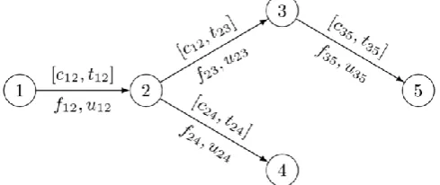
Figure 3: Example of directed and weighted (cost and time) graph representation of a communication network The step from single-objective network flow problem to bi-objective network flow problem is taken by performing the addition of a second set of properties, which is the time of transmission, to every arc of a given network. Considering the same network as in the previous section, the statement of a bi-objective minimum cost flow problem is of the same form of the single-objective minimum cost flow problem, with the addition of a second objective function. The problem can be stated as follows:
(3)
The second objective function is also subject to the same capacity constraint and the flow conservation constraint as the first objective function.
A feasible solution of the linear problem is said to be a non-dominated solution if there does not exist any other feasible solution , such that:
(4) with strict inequality in at least one of k inequalities. Solving the linear problem means finding the set of all non-dominated solutions of the linear problem.
III. METHODOLOGY
Page 53 www.ijiras.com | Email: [email protected] the previous one. in this part, the steps, and description of the
algorithm that was used are given. A. SIMPLEX ALGORITHM
This algorithm is a primal simplex algorithm that solves the following Linear Programming problem:
(5)
This is a two-phase algorithm. In Phase I, the algorithm finds an initial basic feasible solution by solving an auxiliary linear programming problem (see Appendix 1 Phase I). The objective function of the auxiliary problem is the linear
penalty function , where , is
defined by:
(6)
The penalty function measures how much a point x violates the lower and upper bound conditions. The auxiliary problem that is solved is the following:
(7) The original problem (equation 5) has a feasible basis point iff the auxiliary problem (equation 7) has a minimum optimal value of 0. The algorithm finds an initial point for the auxiliary problem (equation 7) using a heuristic method that adds slack and artificial variables. Then, the algorithm solves the auxiliary problem using the initial (feasible) point along with the simplex algorithm. The solution found is the initial (feasible) point for Phase II.
In Phase II, the algorithm applies the simplex algorithm using the initial point from Phase I to solve the original problem (equation 5). The algorithm tests the optimality condition at each iteration and stops if the current solution is optimal. If the current solution is not optimal, the following steps are performed:
The entering variable is chosen from the non-basic variables and the corresponding column is added to the basis.
The leaving variable is chosen from the basic variables and the corresponding column is removed from the basis.
The current solution and objective value are updated
The algorithm detects when there is no progress in Phase II process and it attempts to continue by performing bound perturbation [2]
B. BI-OBJECTIVE ALGORITHM
This section presents the principle of the algorithm developed for solving bi-objective optimization problems formulated in 2.3 (Equation 3 or 8)
(8)
In the single objective network simplex, each basic feasible set is represented by a tree given by the set of basic arcs that have a flow . All the other non-basic arcs have a flow with value of either or . In each step of the algorithm, a non-basic arc is chosen to enter the basis, resulting in a cycle that can be used to determine the arc that leaves the basis.
In the bi-objective case of the problem, the algorithm starts by finding the optimal solution for one of the objective functions using the weighted-sum of the two objective functions, in order to find an initial solution to the multi-objective problem. This new multi-objective function is given by
where has to be given. Here, we take in order to obtain a optimal solution which minimizes only , the first objective function. Then the solution is used as the initial solution for the multi-objective problem. Since there are two components ( and ) associated with each arc (the time and the cost of transmission) in the network, the reduced costs for each arc also consist of two components and . The reduced cost of a given arc , according to Eusébio and Rui [4], is defined as:
(9) Accordingly, the reduced time of a given arc is defined as:
(10) with , , , and being the dual variables (often called potentials) associated with the vertices and . For all arcs in the basis, and . To find all the reduced costs, and the rduced times, we solve the following systems of equations:
(11) And
(12) Then we can use equation 9 and 10 to compute the reduced costs and times.
To find the entering arc, we calculate for each non-basic arc, the ratio:
(13)
Where and N represents
the set of non-basic columns of , the matrix of the constraints.
Page 54 www.ijiras.com | Email: [email protected] simplex pivot operation and one of the candidate arcs is
removed from the candidate set and enters the basis, with an arc leaving the basis. By performing multiple iterations, the algorithm iteratively finds the set of efficient solutions, until the optimal solution for the second objective function is reached, that being the criteria for the algorithm to stop. The complete algorithm is summarized in appendix 2.
IV. RESULTS A. AN ILLUSTRATIVE EXAMPLE
This section aims to report the results for a better understanding of the algorithm behaviour. The algorithm has been implemented using the MATLAB programming language.
An application of the algorithm to a bi-objective minimum cost flow problem. A graphical representation of the network problem used can be seen in Figure 4. The network has 10 nodes, 19 arcs, one source node (node 1) and one sink node (node 10). We then need to send 15 units of data from node 1 to node 10 minimizing at the time, the cost and the transmission of data through the network. The algorithm looks for the path to achieve this.
The algorithm starts by finding the initial solution for the problem using the weighted-sum method presented previously. The solution, illustrated in Figure 5 is the optimal solution for the first objective function . The arcs in the basis are coloured in blue.
Figure 4: Example of a bi-objective network optimization problem
Figure 5: Path minimizing the cost of transmission: z1 = 418 and z2 = 531
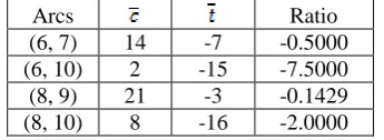
To find the entering arc, the reduced costs ratios are computed for each arc that is not in the basis and that meets the criteria for entering the basis.
Arcs Ratio
(6, 7) 14 -7 -0.5000
(6, 10) 2 -15 -7.5000
(8, 9) 21 -3 -0.1429
(8, 10) 8 -16 -2.0000
Table 1: Reduced costs and and the reduced costs ratios for the candidate arcs
The computed ratios and the reduced costs used to select the entering arc are presented in Table 1. The arc with the lowest reduced cost ratio is the selected one for entering the basis. With this information, the algorithm performs a simplex pivot operation, requesting that the arc (6, 10) is the entering variable.
Figure 6: Iteration 1 z1 = 420 and z2 = 516
Figure 6 shows the graph with the solution obtained from the first iteration of the algorithm.
The algorithm continues the iterations until the value of the second objective function reaches its global optimum. In Figures 7-14 below we show the following iterations of the algorithm.
To have a better compromise between the total cost and time of transmission, the algorithm looks for the arc which will reduce the total time of transmission and increase the total cost of transmission. Therefore, the arc leaves the basis and the arc enters in the basis set of arcs (see Figure 7).
Figure 7: Iteration 2 z1 = 424 and z2 = 502
Page 55 www.ijiras.com | Email: [email protected] Figure 8: Iteration 3 z1 = 430 and z2 = 492
Here, the arc enters in the basis set, while arc leaves (see Figure 9)
Figure 9: Iteration 4 z1 = 452 and z2 = 466
In the fifth iteration, the arc enters in the basis set, while arc leaves (see Figure 10)
Figure 10: Iteration 5 z1 = 468 and z2 = 450
In the iteration 6, the arc enters in the basis set, while arc leaves (see Figure 11)
Figure 11: Iteration6 z1 =492andz2 =442
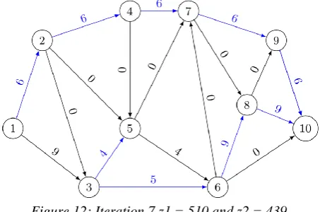
In the iteration 7, only the amounts of flows and change in order to minimize the objective function while increasing the objective function (see Figure 12)
Figure 12: Iteration 7 z1 = 510 and z2 = 439
Here, we observe that for both iterations 7 and 8, represented in figure 12 and 13, the values of the objective functions and do not change even if the basis for each solution is different.
Figure 13: Iteration 8 z1 = 510 and z2 = 439
After the ninth iteration (Figure 14), we obtain the set of path and amount of flow to transfer to jointly minimize the time and the cost of transmission.
Figure 14: Iteration 9 z1 = 524 and z2 = 438
B. COMPUTATIONAL EXPERIMENTS
Page 56 www.ijiras.com | Email: [email protected] obtained from the 2015 final report of ARCEP, the regulatory
authority for electronic communications and stations in Burkina Faso [3,14].
The experiments were done in a Personal Computer equipped with an Intel Core i5 processor 2.5GHz with 6GB of RAM and runs under OS X operating system.
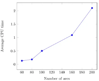
In Table 2, the average CPU time (in second) the algorithm takes to find the optimal solution for different numbers of nodes and arcs are presented.
Nodes Arcs CPU Time(s)
20 60 0.13
20 80 0.17
20 100 0.18
40 120 0.56
40 160 0.77
40 200 1.09
60 180 2.14
Table 2: Results for different sets of network instances
Figure 15: The average CPU time (s) increases quadratically as the number of nodes increases
Figure 16: The average CPU time increases quadratically as the number of arcs increases
We remark from the results that:
When the number of nodes is fixed while increasing the number of arcs, the average CPU time increases significantly.
The CPU time depends mostly on the number of arcs of the network to optimize.
V. CONCLUSION
In this paper, we presented a new method for solving bi-objection linear programming problems based on the simplex method. An introduction to the fundamental concepts of multi-objective optimization and network flows and a short literature review of the current work for multi-objective minimum cost flow problems was presented.
The main characteristic of the algorithm is related to the way the optimum solution is found without destroying the network structure of the problems. Network flow problems, specifically minimum cost network flow problems, are a type of optimization problems that can model many real-world problems even if they do not present a network structure. The algorithm could then be applied in the optimization of transportation systems, communication systems, vehicle routing, production planning, and cash flow analysis. According to our computational results, when the number of nodes is fixed while increasing the number of arcs, the average CPU time increases significantly. This means that the CPU time depends mostly on the number of arcs of the network to optimize.
However, the algorithm is only applicable to problems of optimizing linear objective functions of several variables subject to a set of linear equality or inequality constraints. The algorithm can’t be applied if the objective functions or constraints are not linear. This should be considered as an avenue for future development. Also, to apply the algorithm to practical decision problems in real-time remains a challenging task. Another important issue is to extend the method to more than two objectives.
This research was supported by the Pan African University through the Institute for Basic Sciences, Technology, and Innovation.
ACKNOWLEDGEMENTS
This research was supported by the Pan African University through the Institute for Basic Sciences, Technology, and Innovation.
REFERENCES
[1] Al-Shehri, S. M., Loskot, P., Numanoglu, T., and Mert, M. (2017). Common Metrics for Analyzing, Developing and Managing Telecommunication Networks. pages 1– 51.
[2] Applegate, D. L., Bixby, R. E., Chvatal, V., and Cook, W. J. (2006). The traveling salesman problem: a computational study. Princeton university press.
Page 57 www.ijiras.com | Email: [email protected] [4] Eusébio, A. and Rui, J. (2009). Finding non-dominated
solutions in bi-objective integer network flow problems. Computers & Operations Research, 36:2554–2564. [5] rey, , u fle, , mrich, , and enz,
Efficient information flow maximization in probabilistic graphs. IEEE Transactions on Knowledge and Data Engineering, 30(5):880–894.
[6] Goryczak, W., Pióro, M., and Tomaszewski, A. (2005). Telecommunications network design and max-min optimization problem. Journal of telecommunications and information technology, pages 43–56.
[7] Gounaris, C. E., Rajendran, K., Kevrekidis, I. G., and Floudas, C. A. (2016). Designing networks: A mixed-integer linear optimization approach. Networks, 68(4):283–301.
[8] Manpreet, S. and Priyanka, D. (2014). A Novel Approach to Minimize End-to-End Delay in Wireless Sensor Net- work. International Journal of Wireless Communications and Networking Technologies, 3(3):2–5.
[9] Marler, R. T. and Arora, J. S. (2010). The weighted sum method for multi-objective optimization: new in- sights. Structural and multidisciplinary optimization, (41(6)):853–862.
[10]P. L. Yu, M. Z. (2016). Linear Multiparametric Programming by Multicriteria Simplex Method. Management Science, 23(2):159–170.
[11]Pike-burke, C. (2018). Multi-Objective Optimization. Technical report, Lancaster University.
[12]Seiford, L. and Yu, P. L. (1979). Potential solutions of linear systems: The multi-criteria multiple constraint levels program. Journal of Mathematical Analysis and Applications, 69(2):283–303.
[13]Sifaleras, A. (2013). Minimum cost network flows: Problems, algorithms, and software. Yugoslav Journal of Operations Research, 23(1):3–17.
[14]Sylvestre, O. (2004). Analyse de la situation de la téléphonie rurale au Burkina Faso, Institut Panos Afrique de l’Ouest
APPENDIX 1: SIMPLEX ALGORITHM The typical simplex tableau is written as:
z x1 x2 . . . xn RHS 0 a11 a12 . . . a1n b1 0 a21 a22 . . . a2n b2
. . . . .
0 am1 am2 . . . amn bm 1 am+1,1 am+1,2 . . . am+1,n bm+1
where , if this is a max problem, and
, if it is a min problem. Table 3: Simplex tableau GENERIC SIMPLEX PIVOT FOR ROW R:
P1: Choose entering variable any with
P2: Choose as leaving variable any with , and
P3: Perform a pivot on entry
INITIALIZE:
Perform a standard Gauss-Jordan reduction of the original equality system. If a redundant row is found delete it, and if an inconsistent row is found STOP, the linear program is infeasible.
PHASE I:
For row while do the following:
Attempt a generic simplex pivot.
If Step P1 fails, then STOP, the linear program is infeasible.
If Step P2 fails pivot on element , go to the next row.
If neither P1 or P2 fails, perform the pivot and repeat. When rows have been successfully processed, the linear program is feasible.
PHASE II:
For row do the following:
Attempt a generic simplex pivot.
If Step P1 fails, then STOP, the current solution is optimal.
If Step P2 fails STOP, the linear program is unbounded.
If neither P1 or P2 fails, perform the pivot and repeat.
APPENDIX 2: BI-OBJECTIVE SIMPLEX ALGORITHM INPUT:
A bi-objective Linear Programming problem (LP) of the
form .
PHASE I:
Solve the auxiliary LP to
get optimal solution .
if then
stop there are no feasible solutions. Else
Define B to be the optimal basis. Go to Phase II.
PHASE II:
Define
Solve the LP for
using initial basis B. PHASE III:
Page 58 www.ijiras.com | Email: [email protected] Perform a simplex pivot on row , column .
RETURN:
A sequence of and optimal basic feasible solution.