COMPARISON OF OPTIMIZATION TECHNIQUES OF INPUT
PARAMETERS IN WIRE ELECTRICAL DISCHARGE MACHINING
Avinash K
1, R Rajashekar
2& B M Rajaprakash
3I. INTRODUCTION
Wire EDM (Electric Discharge Machining) is a thermo electrical process in which material is eroded by a series of sparks between the work piece and the wire electrode (tool). The part and wire are immersed in a dielectric (electrically non-conducting) fluid which also acts as a coolant and flushes away debris. The movement of wire is controlled numerically to achieve the desired three dimensional shapes, surface finish and high accuracy of the work piece. In this process, there is no contact between work piece and electrode, thus materials of any hardness can be cut as long as they can conduct electricity. Whereas the wire does not touch the workpiece, so there is no physical pressure imparted on the workpiece and the amount of clamping pressure required to hold the workpiece is minimal. Although electrical conductivity is an important factor in this type of machining, some techniques can be used to increase the efficiency in machining of low electrical conductive materials. The heat of each electrical spark, estimated at around 15,000° to 21,000° Fahrenheit, at this temperature erosion of workpiece takes place and hence cutting can be achieved by moving wire or base on which work is mounted in desired work path. This process has been widely used in aerospace, nuclear and automotive industries, to machine precise, complex and irregular shapes in various difficult to machine electrically conductive materials. Wire EDM process is also being used to machine a wide variety of miniature and micro-parts made of metals, alloys, sintered materials, cemented carbides, ceramics and silicon. These characteristics makes Wire EDM a process which has remained as a competitive and economical machining option fulfilling the demanding machining requirements imposed by the short product development cycles and the growing cost pressures. The working principle is shown in Figure 1.
The most important performance measures in Wire EDM are Metal Removal Rate (MRR) and Surface Roughness (Ra). They depend on machining parameters or process parameter or input parameter like discharge current, pulse on time, pulse off time, wire speed, wire tension, servo voltage and dielectric flow rate.
Figure 1 Schematic diagram of working principle of Wire EDM
1Research scholar, Department of Mechanical Engineering, University Visvesvaraya College of Engineering, Bangalore University, K R
circle Bengaluru, Karnataka, India – 560001
2Assistance Professor, Department of mechanical engineering, University Visvesvaraya College of Engineering, Bangalore University, K R
circle Bengaluru, Karnataka, India – 560001
3Professor and Chairman, Department of mechanical engineering, University Visvesvaraya College of Engineering, Bangalore University,
K R circle Bengaluru, Karnataka, India – 560001
International Journal of Latest Trends in Engineering and Technology
Vol.(8)Issue(4-1), pp.149-155
DOI: http://dx.doi.org/10.21172/1.841.26
e-ISSN:2278-621X
Abstract –Wire EDM is a non-traditional machining method primarily used for machining hard metals or those that would be impossible to machine with traditional techniques. The non-contact machining technique has been continuously evolving from a mere tool and dies making process to a micro-scale application. In this research paper, the machining of High Speed Steel (HSS) material using Wire Electric Discharge Machining (WEDM) with Brass as a wire electrode has been carried out. The pulse on time, pulse off time and servo voltage were selected as control process parameters of Wire EDM. Both Taguchi and Response Surface Method (RSM) techniques were applied to determine optimized process parameter to maximize Material Removal Rate (MRR) and minimize Surface Roughness (Ra). These techniques were compared based on time, trials and cost concern. The effect of process parameters on MRR and Ra was found by using Analysis of Variance (ANOVA)
Among these machining parameters, Pulse on time, pulse off time and servo voltage have been considered for experimental purpose, as they are the most significant control factors for both maximization of MRR and minimization of Ra (Performance parameter or output parameter). Process parameters are generally controllable machining input factors that determine the conditions in which machining is carried out. These machining conditions will affect the process performance result, which are gauged using various performance measures.
In setting the machining parameters to obtain maximum MRR and minimum Ra, generally the machine tool builder provides machining parameter table. This process relies heavily on the experience of the operators. In practice, it makes very difficult to utilize the optimal functions of a machine owing there are too many adjustable machining parameters. To solve this difficulty, a simple but reliable method based on statistically designed experiments is suggested for investigating the effects of various process parameters on MRR and Ra and determine optimal process settings. There are several optimizing techniques available and among them Taguchi technique and Response Surface Methodology are very efficient, powerful experimental design tools which uses simple, effective and systematic approach for deriving of the optimal machining parameters.
In the present work, both Taguchi method and Response Surface Method (RSM) were applied to determine optimized process parameter to maximize Material Removal Rate (MRR) and minimize surface roughness (Ra). Taguchi technique and RSM have been compared based on the time consumed, cost of operation and number of trials.
II. METHODOLOGY
A. Machine specification and material
The experiments were carried out on a Wire EDM machine (ECOCUT WEDM) to measure MRR value and Mituttoyo Surface Roghness Tester was used to measure Ra value.
The Wire EDM machine tool has following specifications: X Axis Table Travel : 250 mm
Y Axis Table Travel : 350 mm
Z Axis Travel : 200 mm
Max. work piece size : 575 X 835 X 200 mm Max. Work piece wt. : 275 Kg
Main table feed rate : 80 mm/ min
Wire feed rate : 0 - 10 m / min
Wire guide type : Diamond closed
Wire electrode diameter : 0.25mm STD, 0.2mm optional
Input voltage : 310 V to 467 V line to line. i.e . 180 -- 270 V / phase
Output voltage : 415 V line to linei.e . 240 V phase to neutral
Voltage correction rate : 35 V / sec
The de-ionized water is used as dielectric: The Mituttoyo Surface Roghness Tester has following specifications
Measurement range : 350 µm (-200µm to +150µm)
Power system : 2 Way (AC adaptor/rechargeable built in battery).
The sensor movement given to indenter: 4mm
High Speed Steel (HSS) is used as work piece material for the present work due to the reason that HSS cannot be easily machinable by conventional machining techniques as it has high hardness, also it is an important tool material being used in industries. Chemical composition of HSS material is represented in Table 1.
Table 1 Composition of the material
Constituents C Si Ma P S Cr Mo Ni
% Comp 1.364 1.9616 0.456 0.052 0.046 1.921 0.127 0.065
B. Optimization techniques
1. Response Surface Methodology (RSM)
Response surface methodology (RSM) is a collection of mathematical and statistical techniques for empirical model building. By careful design of experiments, the objective is to optimize a response (output variable/performance parameter) which is influenced by several independent variables (input/process parameter). The problem can be approximated as described in smooth functions that improve the convergence of the optimization process because they reduce the effects of noise and they allow for the use of derivative based algorithms.
In this method if the response is well modeled by a linear function of the independent variables, then the approximating function as per the First order model is,
Avinash K, R Rajashekar & B M Rajaprakash
If there is curvature in the system, then a polynomial of higher degree must be used and the corresponding second order model is,
YU = b0 + + + + …. + e (2)
Where ‘i’ is the linear coefficient, ‘j’ is the quadratic coefficient, ‘β’ is the regression coefficient, ‘k’ is the number of studied and optimized factors in the experiment and ‘e’ is the random error. Analysis of variance (ANOVA) has taken into account in order to estimate the suitability of the regression model.
2. Taguchi techniques
Genichi Taguchi, a Japanese scientist, developed a technique. This technique has been widely used in different fields of engineering to optimize the process parameters. The integration of Design Of Experiment (DOE) with parametric optimization of process can be achieved in the Taguchi method. Taguchi’s Signal-to-Noise ratios, (S/N ratios) which are logarithmic functions of the desired output, serve as objective functions for optimization. It helps to learn the whole parameter space with a small number (minimum experimental runs) of experiments. S/N ratios are used to study the effects of control factors and noise factors and to determine the best quality characteristics for particular applications. The optimal process parameters obtained from the Taguchi method are insensitive to the variation of environmental conditions and other noise factors. However, originally, Taguchi method was designed to optimize single-performance characteristics. Optimization of multiple performance characteristics is not straightforward and much more complicated than that of single performance characteristics. The experimental observations are further transformed into a signal-to-noise (S/N) ratio. There are several S/N ratios available depending on the type of characteristics. The characteristic that higher value represents better machining performance, such as MRR, is called higher is better (HB). Inversely, the characteristic that lower value represents better machining performance, such as surface roughness, is called lower is better (LB). Therefore, ‘HB’ for the MRR and ’LB’ for the Ra were considered for obtaining optimum input process parameter.
The loss function (L) for objective of HB and LB is defined as follows:
LHB= (3)
LLB= (4)
Where ‘yMRR’, and ‘yRa’ are response for material removal rate and surface roughness, and ‘n’ denotes the experiment number.
The S/N ratio can be calculated as a logarithmic transformation of the loss function as,
S/N ratio for MRR = -10 log10 (LHB) (5)
S/N ratio for Ra = -10 log10 (LLB) (6)
III. EXPERIMENTATION
A. Selection of process parameters and their levels
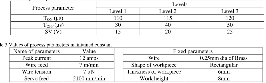
Among all process parameters three parameters such as pulse on time (TON), pulse off time (TOFF) and servo voltage (SV) are
varied during experimentation in three levels, the range of which are found by trial and error method. Table 2 shows parameters selected and their levels. Apart from these parameters there are also other parameters and factors which also have significant effect on performance parameters which are shown in Table 3. They are kept constant to minimize their effects
Table 2 Levels of process parameters
Process parameter Levels
Level 1 Level 2 Level 3
TON (µs) 110 115 120
TOFF (µs) 30 40 50
SV (V) 15 20 25
Table 3 Values of process parameters maintained constant
Name of parameters Value Fixed parameters
Peak current 12 amps Wire 0.25mm dia of Brass
Wire feed 7 m/min Shape of workpiece Rectangular
Wire tension 7 µN Thickness of workpiece 6mm
Servo feed 2100 mm/min Work height 8mm
B. Experimental design using Taguchi’s technique
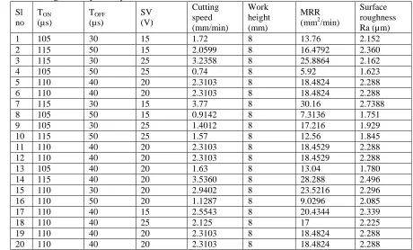
MRR= Cutting speed x work height (7) Where ‘cutting speed’ was measured during each trial
The experimental measured value of MRR and Ra their S/N ratios, calculated using equation (5) and (6) respectively are presented in Table 4.
Table 4: L9 orthogonal array, experimental results and S/N ratios
Trial no Ton (µs) Toff (µs) SV (V) MRR (mm2/min)
Surface Roughness Ra (µm)
S/N ratio of MRR
S/N ratio of RA
1 105 30 15 13.76 2.152 22.7724 -6.65685
2 105 40 20 13.04 1.780 22.3056 -5.00840
3 105 50 25 5.92 1.623 15.4464 -4.20637
4 110 30 20 23.5216 2.290 27.4293 -7.19671
5 110 40 25 17 2.225 24.6090 -6.94660
6 110 50 15 10.34 2.123 20.2904 -6.53900
7 115 30 25 25.8864 2.162 28.2614 -6.69711
8 115 40 15 29.04 2.572 29.2599 -8.20542
9 115 50 20 14.3832 2.036 23.1571 -6.17556
C. Experimental design using Response Surface Methodology (RSM)
In RSM L20 orthogonal array was chosen. It consists of 20 rows corresponding to the number of experiments with three columns of process parameters. Here same selected process parameters for same three levels as used in Taguchi’s technique are varied. Face centered central composite design was adopted to design the experiments as shown in Table 5. RSM was used to develop second order regression equation which gives relation between process parameters (TON, TOFF and SV) and
performance parameters (MRR or Ra).
Table 5: L20 orthogonal array and experimental results for RSM
Sl no TON (µs) TOFF (µs) SV (V) Cutting speed (mm/min) Work height (mm) MRR (mm2/min)
Surface roughness Ra (µm)
1 105 30 15 1.72 8 13.76 2.152
2 115 50 15 2.0599 8 16.4792 2.360
3 115 30 25 3.2358 8 25.8864 2.162
4 105 50 25 0.74 8 5.92 1.623
5 110 40 20 2.3103 8 18.4824 2.288
6 110 40 20 2.3103 8 18.4824 2.288
7 115 30 15 3.77 8 30.16 2.7388
8 105 50 15 0.9142 8 7.3136 1.751
9 105 30 25 1.4012 8 17.216 1.929
10 115 50 25 1.57 8 12.56 1.845
11 110 40 20 2.3103 8 18.4529 2.288
12 110 40 20 2.3103 8 18.4529 2.288
13 105 40 20 1.63 8 13.04 1.780
14 115 40 20 3.5360 8 28.288 2.496
15 110 30 20 2.9402 8 23.5216 2.296
16 110 50 20 1.1287 8 9.0296 2.085
17 110 40 15 2.5543 8 20.4344 2.339
18 110 40 25 2.125 8 17 2.225
19 110 40 20 2.3103 8 18.4824 2.288
20 110 40 20 2.3103 8 18.4824 2.288
IV. RESULTS AND DISCUSSION
A. Optimum parameters using Taguchi’s analysis
Avinash K, R Rajashekar & B M Rajaprakash
(Level 3), TOFF=30 µs (Level 1) and SV=20 V (Level 2), which results in maximum MRR and similarly factors at level TON
=105 µs (Level 1), TOFF=50 µs (Level 3) and SV= 25 V (Level 3) which results in minimum Ra.
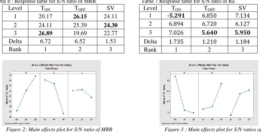
Table 6 : Response table for S/N ratio of MRR Table 7 Response table for S/N ratio of Ra
Level TON TOFF SV
1 -5.291 6.850 7.134
2 6.894 6.720 6.127
3 7.026 5.640 5.950
Delta 1.735 1.210 1.184
Rank 1 2 3
Figure 2: Main effects plot for S/N ratio of MRR Figure 3 : Main effects plot for S/N ratios of Ra
B. Confirmation experiment for results obtained from Taguchi
The optimal combination of process parameter obtained from analysis of results are verified by conducting the experiments for those combinations and compared with the value predicted by using equation 7 for MRR and Ra separately. Both experimental and predicted values for optimum parameter to get maximum MRR and minimum Ra are shown in Table 8 and Table 9 respectively.
) (7)
Where =Total mean of S/N ratio, = Mean of S/N ratio at optimum level of each parameter p = Number of main machining parameters (Here 3)
Table 8 Confirmation experiment for MRR Table 9 Confirmation experiment for Ra
Optimal machining parameter
Prediction Experimental
Level TON 1, TOFF 3, SV 3
TON 1, TOFF 3,
SV 3 S/N Ratio for
Ra -4.074 -4.2063
Ra 1.5984 1.623
% error 1.53
C. Optimum parameters using Response Surface Methodology (RSM)
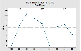
Based on Analysis of Variance (ANOVA) Figures 4 and 5 show the effect of three process parameters on MRR and Ra respectively, indicating that TON is the most affecting parameter for both MRR and Ra, while pulse off time and Servo voltage
are less significant for both MRR and Ra.
Figures 6 and 7 show optimization plot using desirability approach for MRR and Ra respectively. Main effect plots, optimization plots and surface plots are generated using MINITAB 16.
Desirability approach has been used for finding out the optimum values of the process parameter in order to get the maximum value of MRR and minimum value of Ra. It is clear from the Figure 6 that highest value of MRR 31.4975 mm2/min, is obtained for the combination of Ton = 115 µs, TOFF = 30 µs and SV = 15 volt. It is clear from the Figure 7 that lowest value of
Ra 1.6228 µm is obtained for the combination of Ton = 105 µs, TOFF = 50 µs and SV = 25 volt. The results obtained are with
the composite desirability of 1.000.
Level TON TOFF SV
1 20.17 26.15 24.11
2 24.11 25.39 24.30
3 26.89 19.69 22.77
Delta 6.72 6.52 1.53
Rank 1 2 3
Optimal machining parameter
Prediction Experimental
Level TON 3, TOFF 1, SV 2
TON 3, TOFF 1,
SV 2 S/N Ratio for
MRR 29.8856 29.5192
MRR 31.2197 29.92
Figure 4: main effects plot for data means of MRR Figure 5: main effects plot for data means of Ra
Figure 6: Optimization plot for MRR Figure 7: Optimization plot for Ra
D. Confirmation experiments for results obtained from RSM
The optimal combinations obtained from the analysis of results are verified by conducting the experiments for those combinations. The mathematical model expressing the relation between process parameters and performance parameters (MRR and Ra) was generated using MINITAB 16. This equation called as regression equation was used to predict the performance parameter value for the optimal combinations. Both experimental and predicted values for optimum parameters to get maximum MRR and minimum Ra are shown in Table 10.
For MRR and Ra, regression equation are given in equation 8 and 9 respectively
(8)
(9)
Table 10: Confirmation experiments for MRR and Ra Table 11: Comparison of results of RSM and Taguchi
Respo nse
Experimental results
Taguchi’s RSM
Experi mental
predicte d
Experim ental
Predict ed
MRR 29.92 31.2197 30.16 31.497
Ra 1.623 1.5984 1.623 1.6228
MRR = 191 - 6.95 Ton + 6.18 Toff + 3.15 SV + 0.0461 Ton*Ton - 0.03236 Toff*Toff - 0.0318 SV*SV - 0.0382 Ton*Toff - 0.0213 Ton*SV + 0.0038 Toff*SV
Ra = -77.3 + 1.332 Ton + 0.0423 Toff + 0.353 SV - 0.00551 Ton*Ton - 0.000882 Toff*Toff + 0.00025 SV*SV + 0.000042 Ton*Toff - 0.00373 Ton*SV + 0.000378 Toff*SV
Resp onse
Optimized value of
input parameter Predict
ed
Expe rime
ntal % Error
TON TOFF SV
MRR 115 30 15 31.497 30.16 4.43
Avinash K, R Rajashekar & B M Rajaprakash
E. Comparison of Taguchi technique and RSM
Experimental and predicted results for both Taguchi’s and RSM techniques based on optimal parameter combination is shown in Table 11. Also it was observed that different optimum parameter combination is obtained from Taguchi and RSM for MRR, while same combinations obtained for Ra. It can be observed from the Table 11 that the MRR and Ra values obtained from both techniques are very close to each other.
V. CONCLUSIONS
In this study an attempt was made to determine the values of optimum process parameter to maximize the material removal rate and minimize the surface roughness in Wire EDM. Both RSM and Taguchi techniques are applied for optimization. From the above work it can be concluded that
Both techniques have revealed comparable results.
The results obtained from both RSM and Taguchi techniques are very close for the considered combination of optimal of process parameters.
Though the optimal process parameters combinations for maximization of MRR are different from RSM and Taguchi technique, the MRR obtained is close to each other.
Optimal process parameter combinations for minimization of Ra are same from RSM and Taguchi technique and results are close to each other.
As the time and experimental trials required by RSM is much more than that of Taguchi method also results obtained from both methods are very close, the Taguchi technique (L9) is more suitable than RSM (L20) for optimization of parameters of HSS material in the chosen experimentation.
It is clear that Pulse on time has greater influence on maximization of MRR and minimization of Ra. Also, pulse off time and servo voltage influence the MRR and Ra to a smaller extent.
Customized values of MRR and Ra can be obtained by solving equation obtained from desirability approach.
REFERENCES
[1] S. S. Mahapatra& Amar Patnaik (2006), Optimization of wire electrical discharge Machining (WEDM) process parameters using Taguchi method, J. of the Braz. Soc. Of Mech. Sci. & Eng. Vol. 28, No. pp-422-429
[2] PragyaShandilyaa*, P.K.Jainb N.K. Jain (2012), Parametric optimization during wire electrical discharge machining using response surface methodology, Procedia Engineering 38, pp 2371-2377
[3] R.Pandithurai, I. Ambrose Edward (2014), Optimizing surface roughness in Wire-EDM using machining parameters, International Journal of Innovative Reaserch in Science, Engineering and Technology, vol. 3, Special issue 3, pp 1321-1324
[4] G. Venkateswarlu, P. Devaraj (2015), Optimization of Machining Parameters in Wire EDM of Copper Using Taguchi Analysis, International Journal of Advanced Materials Research Vol. 1, No. 4, 2015, pp. 126-131
[5] Vikram Singh, S.K, Pradhan (2014), Optimization of WEDM parameters using Taguchi technique and Response Surface Methodology in machining of AISI D2 Steel, Procedia Engineering 97, pp 1597-1608
[6] Pratik A. Patil, C.A. Waghmare, Optimization of process parameters in Wire EDM using RSM, Proceedings of 10th International Conference, pune,
India, ISBN: 978-93-84209-23-0
[7] K. Kumar, R Ravikumar (2013), Modelling and Optimization of Wire EDM process, International Journal of Madern Engineering Research, Vol. 3, Issue. 3, pp-1645-1648.
[8] Neeraj Sharma, Rajesh Khanna, Rahul Dev Gupta (2015), WEDM process variables investigation for HSLA by response surface methodology and genetic algorithm, Engineering Science and Technology, an International Journal 18, pp 171-177