I J E N S
2010 IJENS June IJENS © -IJECS 7373 -3 0 1026
Control Using Sliding Mode Of the Magnetic
Suspension System
Yousfi Khemissi
Department of Electrical Engineering Najran University Kingdom Saudi Arabia e-mail : [email protected], e-mail : [email protected]
Abstract - This paper presents a proposition of sliding mode position controller of the magnetic suspension ball system . The magnetic suspension system (MS S ) is a mechatronic system already acknowledged and accepted by the field experts. The design of a controller keeping a steel ball suspended in the air. In the ideal situation, the magneti c force produced by current from an electromagnet will counteract the weight of the steel ball. Nevertheless, the fixed electromagnetic force is very sensitive, and there is noise that creates acceleration forces on the steel ball, causing the ball to move into the unbalanced region. The main function of the sliding mode control (S MC) Controller is to maintain the balance between the magnetic force and the ball's weight. The proposed controller guarantee the asymptotic regulation of the states of the system to their desired values.
Complete mathematical models of the electrical, mechanical and magnetic suspension system are also developed. The design and simulations are performed under a Matlab/S imulink models computer package, allows us to examine the performance of this technique: improvement of the stability and the dynamic response.
Index Term-- Magnetic suspension system - S liding Mode Control – S tability and performance - simulation.
1. INT RODUCT ION
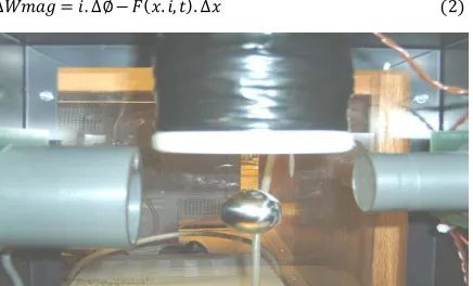
The predictive control has become a very impo rtant area of research in recent years. Magnetic suspension systems shown in Fig.1. have received increasing attention recently, due to their practical importance in many engineering systems. Few of the presented schemes, however, have been realized in industrial application so far [1]. They are becoming popular in many applications, such as h igh-speed passenger trains, frictionless bearings, levitation of wind tunnel models, vibration isolation of sensitive machinery, levitation of molten metal in induction furnaces, and levitation of metal slabs during manufacturing [2-5]. Magnetic levitation systems are nonlinear and open loop unstable. This has led to a significant demand for control technologies for use in magnetic suspension systems. Feedback linearizing control is an approach to the design of nonlinear controllers [7,8]. Recently, many researchers have applied this approach to magnetic suspension systems [9-10], especially in cases where magnetic suspension systems are required to operate under large variation of the air gap. High performance control of a magnetic suspension system of attractive type in the presence of parameter uncertainties is of particular interest. To achieve robustness of the control system, sliding mode control . The object of this model is to keep a metal ball suspended in mid-air by adjusting the field strength of an electromagnet. The electromagnet current may be increased until the magnetic force produced is equal
to or greater than, the gravitational force acting on the ball. Variations in the electromagnet current cause the ball to either fall when current is decreasing or be attached to the electromagnet when current is increasing. The feedback path control introduced aims to stabilize the ball when current disturbance occurs.
2. THE MAT HEMAT ICAL MODEL OF T HE
ELECT ROMAGNET IC SUSPENSION SYST EM One can build the mathematical model of the levitation system by writing appropriate differential equations in accordance to the typical mechanical- and electrical
principles. The way the components are appreciated in the approaching mode can lead to simpler or more complex alternatives.
The formula for the energetic balance within the system is:
Where, the terms represent the variation of the electrical energy (ΔWelec), the variation of the mechanical energy (ΔWmec), the variation of the thermal energy (ΔWther) and the variation of the magnetic energy (ΔWmag).
The variation of the magnetic energy when the magnetic fluxes are varying and bodies are moving within the magnetic field is:
Fig. 2. Force diagram
The electromagnetic levitation force can be determined using the theorems of the generalized forces [11]:
The specific magnetic energy of a coil is:
The coil inductivity L is a nonlinear function depends upon the position “x” of the ferromagnetic ball in accordance to the relationship (5) [12] defined as:
where L1 is a system parameter.
In the given context, one can particularize the dynamic model of the levitation system for each mode of calculating the inductivity.
Let the states and the control input be chosen such that x1=x, x2=v, x3=i , u=e . This dynamic model of system is expressed by the equations (7) to (9) :
Where, x – represents the ball position with respect to the reference position; v – represents the speed of the ball; i – represents the current intensity in the electromagnet winding; e – represents the supply voltage of the coil; R – represents the resistance of the electromagnet winding; L – represents the winding inductivity; g – represents the gravity acceleration (which is constant); m – represents the ball mass.
A development of the defined mathematical model can be achieved based on the system status, if considering the status variables X=(x1 x2 x3)T =(x v i)T and u = e .
Using the typical systems linearization principle (the expansion in Fourier series and the preservation of the first order terms), one can linearize the acquired nonlinear model.
3. THE ELECT RICAL MODEL
The formula for the relationship between voltage and current of the electromagnet coil is represented by (8) can be written as :
Where L(x) is represented by (5), after derivation of L(x) are:
Orthe supply voltage of the coil U is:
Where
Thus, the state-space model of the magnetic levitation system can be written as:
Let x01, x02, and x03 be the desired values of x1, x2, and x3, respectively. Note, from (14), that the equilibrium point for the system is X0 = (x01 0 x03)T, where
x03 =(g.m/C)1/2.x01. Therefore, one may conclude that x2d is equal to zero.
The objective of the control schemes is to drive the states x1, x2, and x3 to their desired constant values x1ref, x2ref, and x3ref, respectively.
4. DESIGN OF SWIT CHING SURFACE
The state-space model of the magnetic levitation system (14) will be used in the design of the SMC schemes. Here the switching surface with integral operation for the sliding-mode position controller is designed as follows [2,3]. Now, consider the following nonlinear change of coordinates:
Where x1ref is reference trajectory, the dynamic model of the
magnetic levitation system in the new coordinates system can be written as :
Differentiating (16) with respect to time we can write the following:
Substituting (14) into (17)
It should be noted that the functions f (x) and g(x) correspond in the original coordinates to the following functions, respectively:
( )
( )
( ) ( )
()
,
(
)
̇ ̇ ( )
̇ ( )
̇ ̇
̇ ( ( ))
( )
̇ ( ̇) ( ̇)
̇ * ( ( ) ) ( )+
*( ) +
I J E N S 2010 IJENS June IJENS © -IJECS 7373 -3 0 1026
To establish the sliding mode disturbance estimator, we define the switching surface function S as :
Where σ1 and σ2 are positive scalars represents the feedback gain to be designed so that the error dynamics will have the desired response while the system is free of uncertainties and disturbances .
Note that the choice of the switching surface S guarantees that y1 = x1 − x1ref converges to 0 as t→∞ when we have sliding surface S=0, the output x1 is governed after such finite amount of time by the second- order differential equation. Thus the output y1(t) = x1(t) will converge asymptotically to 0 as t →∞ because σ1 and σ2 are
positive scalars. Since x1 converges to zero, then x2 and x3 will converge to zero as t→∞. Thus x1, x2, and x3 will also converge to their desired values as t→∞.
Therefore, it can be concluded that the static sliding mode controller given by (19) guarantees the asymptotic convergence of the states x1, x2, and x3 to their desired values as t→∞.
Defining our sliding condition [13], the control strategy adopted here will guarantee a system trajectory move toward and stay on the sliding surface S = 0 from any initial condition if the following condition meets .
.
where is a positive constant that guarantees the system trajectories hit the sliding surface in finite time [13].
Using a sign function often causes chattering in practice. One solution is to introduce a boundary layer around the switch surface [14].
Differentiating (19) with respect to time we can write the following:
The solution of this equation ( 21 ) and (22) gives us the control law of the tension.
Where the switching surface S can be written as a function of x1, x2, and x3such that
The specifications and system parameters of the proposed magnetic suspension system are listed in Table I.
T ABLE I
SP ECIFICATIONS AND SYSTEM P ARAMETERS OF SYSTEM
parameters Values
Mass of the steel ball M =0.014 kg
Acceleration due to
gravity
G =9.81 m/s2
Equilibrium distance X01=0.009 m
Equilibrium current I0 =1.5 A
Force constant K=m.g.(x01/i0)2=4.94410-6
Nm2/A2
Coil Resistance R=5.2 Ω
Coil Inductance L1=0.027 H
Coil Inductivity when the ball is absent
L0 =2.k/x01 =0.0011H
5. SIMULAT ION RESULT S
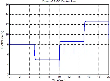
The proposed control scheme is simulated using MATLAB. Magnetic suspension system and force control are shown in Figs. 1-2; control using sliding mode of the magnetic suspension system is shown in Fig. 3;
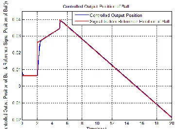
Results of the SMC: Controlled Output Position where the random disturbance (reference trajectory) in form case.1 and sinusoidal case.2, sign builder case.3 and pulse generator disturbance in form case.4 with SMC controller are shown in Figs. 4,10-11-12. The control law and sliding surface when random disturbance are shown in Figs. 5-6. The current variation i(t) during the disturbance to maintain stable ball is shown in Fig. 7. The two opposing forces applied to the ball (magnetic force f(x,i,t) and gravity force f0) almost identical are shown in Figs. 8-9. the difference between the two forces (Gravity force f0 and Magnetic force) are almost negligible for all cases (1-4) which shows the good of the system with sliding mode control followed the trajectory desire.
6. CONCLUSION
An approach for controlling the magnetic
suspension system based on sliding mode has been presented. The model of the magnetic suspension has been realised using the simple electromagnetic and a steel ball. The simplified mathematical model has been developed. The performance of the SMC controller in trajectory tracking is superior for different disturbance signal in form (Random reference, signal builder or pulse generator ) applied to the ball.
Author believes that the proposed disturbance observer based sliding mode control will widen the uses of the sliding mode control in areas where robustness is required with the less chattering.
Sliding mode control (SMC) enables system stability even for large supply and load variations, gives good dynamic response and has simple implementation. These features make this control technique a valid alternative for standard control approaches like speed and position control. We can also conclude that the performance of the SMC controller in disturbance attenuation is good
REFERENCES
[1] H. K. Khalil, Nonlinear Systems. New Jersey: Prentice Hall, 1996.
Motion Control Stage,” IEEE Trans. Contr. Syst. Technol., Vol. 4, No. 5, pp. 553-564 (1997).
[3] K.Yousfi World Journal of Engineering " Sliding mode control of nonlinear systems using model-error control ". ISSN :1708-5284 -Vol.4 , No.1, 2007.
[4] Yamamura, S. and H., Yamaguchi, “Electromagnet Levitation System by Means of Salient -pole Type Magnets Coupled with Laminated Slotless Rails,” IEEE Trans. Veh. Technol., Vol. 39, pp. 83-87 (1990).
[5] Dahlen, N.J., “Magnetic Active Suspension and Isolation,” S.M. T hesis, Department of Mechanical Engineering, Massachusetts Institute of T echnology, Cambridge, MA (1985).
[6] T rumper, D.L., “Magnetic Suspension Techniques for Precision Motion Control,” Ph.D. Dissertation, Department of Electrical Engineering and Computer Science, Massachusetts Institute of T echnology, MA. (1990).
[7] Meyer, G., R., Su and L.R. Hunt, “Application of Nonlinear T ransformations to Automatic Flight Control,” Automatica, Vol. 20, No. 1, pp. 103-107 (1984).
[8] T rumper, D.L., S.M., Olson and P.K., Subrahmanyan, “Linearizing Control of Magnetic Suspension Systems,” IEEE
Trans. Contr. Syst. Technol., Vol. 5, No. 4, pp. 427-438 (1997).
[9] Charara, A., J., De Miras and B., Caron, “Nonlinear Control of a Magnetic Levitation System without Premagnetization,” IEEE
Trans. Contr. Syst. Technol., Vol. 4, No. 5, pp. 513-523 (1996).
[10] Zhang, F. and K., Suyama, “Nonlinear Feedback Control of Magnetic Levitating System By Exact Linearization Approach,”
Proc. IEEE Conf. Contr. Appl., pp. 267-268 (1995).
[11] T imotin, A., Hortopan, V., Ifrim, A., Preda, M., Lecţii de Bazele Electrotehnicii, EDP Bucureşti 1970
[12] Suspensions magnetiques supraconductrices pour volant d’inertie,
http://lanoswww.epfl.ch/studinfo/courses/cours_supra/levitation /volant_inertie.htm
[13] John Y. Hung, W. Gao and James C. Hung, “Variable Structure Control: A Survey,” IEEE T ransactions on Industrial Electronics, vol.40, no.1, pp.2-21, 1993.
[14] J.J. Slotine and W. Li, Applied Nonlinear Control, Englewood Cliffs, NJ: Prentice-Hall, 1991.
Fig. 5. Control Law where the random disturbance in form
Fig. 6. Sliding Surface where the random disturbance in form
Fig. 7. Current with SMC controller
Fig. 8. Magnetic and Gravity Force with SMC controller Fig. 3. Magnetic suspension system with SMC Controller
I J E N S
2010 IJENS June IJENS © -IJECS 7373 -3 0 1026
Fig. 9. Magnetic , Gravity Force and difference between them with SMC controller
Fig. 10. Controlled Output Position when sinusoidal disturbance in form of Ball with SMC controller
Fig. 11. Controlled Output Position when Signal builder disturbance in form of Ball with SMC controller
Fig. 12. Controlled Output Position when Signal Pulse Generator disturbance in form of Ball with SMC controller