Determination of Distance Between AC Traction Power Centers With A Designed Model Depending on Operational Datas in A 25 Kv AC Railway Line Using Artificial Intelligence Methods

e-ISSN: 2278-067X, p-ISSN: 2278-800X, www.ijerd.com

Volume 13, Issue 11 (November 2017), PP.18-27

Determination of Distance Between AC Traction Power Centers

With A Designed Model Depending on Operational Datas in A 25

Kv AC Railway Line Using Artificial Intelligence Methods

*Mehmet Taciddin Akçay

,

İ

lhan Kocaarslan

1_{Istanbul MetropolitianMunicipility, Diroctorate of Rail Systems, Istanbul, Turkey.} 2

Department of Electrical-Elektronics Engineering, Faculty of Engineering, Istanbul University, Istanbul, Turkey

Corresponding Author:Mehmet Taciddin Akçay

ABSTRACT:-

parameters. While the electrification system is designed, the minimum voltage rating required by the traction force in the course of operation needs to be provided. The maximum value of the voltage drop occurring on the line determined by the distance of traction power centers. This value needs to be kept within certain limits for the continuity of the operation. In this study, the determination of the distance between traction power centers by means of the adaptive neuro-fuzzy inference system (ANFIS), support vector machines (SVM) and artificial neural networks (ANN) for a 25 kV AC supplied railway. The distance value was calculated with regard to the operating data by means of ANFIS, SVM and ANN. ANFIS, SVM and ANN were explained and the results were compared.

Keywords:-

---

Date of Submission: 07 -11-2017 Date of acceptance: 16-11-2017

---I.

INTRODUCTION

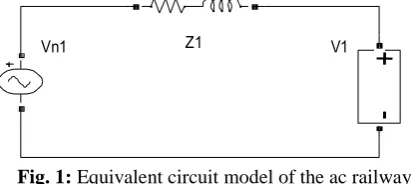
Mostly 25 kV 50 Hz. single-phase supply voltage is used for the traction force system on AC supplied railways. The single-phase supply voltage that the traction force uses is acquired through an interconnected network which has 154 kV phase to phase voltage. Two transformers of 154 kV / 25 kV are present in the substations and the transformers can operate as back-up [1-4]. The equivalent circuit model of the AC railway is presented in Figure 1.

Fig. 1: Equivalent circuit model of the ac railway

The equation regarding the supplying status from a single substation is given with Equation (1) which represents the total impedance from substation Z1 to the vehicle. The impedance values of the feeder cables were also added to Z1. Z1 value changes in accordance with the distance depending on the location of the vehicle. V1 is the voltage of the vehicle, Vn1 indicates the nominal supply voltage, Ivehicleindicates thevehicle current. The maximum traction force of the vehicles in the railway vehicles with a high power consumption can increase to 20 MVA [5-7].

𝑉1= 𝑉𝑛1− 𝐼𝑣𝑒𝑕𝑖𝑐𝑙𝑒 × 𝑅1− 𝐼𝑣𝑒𝑕𝑖𝑐𝑙𝑒 × 𝑅3 (1)

Neutral zones increase the operating capability by allowing to be supplied from different zones. Since the voltage drop occurring on the line and the currents drawn do not reach high values under normal operating conditions, the distances between the supply stations may be longer. As the number of traction supply stations and the efficiency of the traction force system increase, the voltage drop on the line and the losses decrease

[9-Z1

Vn1 V1

₊

-12]. The traction system of the railway vehicle consists of a transformer, a three-phase PWM inverter and an asynchronous engine. In the course of regenerative braking, the asynchronous engine can function as a generator and enables energy transfer. This gain is more effective with the developed power electronics technology. With new research and studies, new traction force converters, various electric equipment used in railway vehicles also undergo a change. The single-line scheme of the traction force supply diagram of an AC supplied railway is displayed in Figure 2.

Fig. 2. Single-Line scheme of the traction force supply diagram

The vehicle traction force (Ftraction) consists of the sum of the resistance force against vehicle motion (Fmotion), slope resistance force (Fslope), curve resistance force (Fcurve) and the multiplication of acceleration and mass of the vehicle, which are given with (2), (3), (4) and (5). In the equations, V is the vehicle speed, m is the vehicle mass, A, B, C are the coefficients related to the vehicle characteristic, g is the gravitational acceleration, γ is the angle of inclination, R is the curve radius, C1, C2 and C3 are the coefficients used to calculate the curve force. In equation (5), the acceleration-mass (ma) value expresses the net force that affects the vehicle. The power equation of the vehicle is given with regard to the traction force and vehicle speed by Equation (6).

𝐹𝑚𝑜𝑡𝑖𝑜𝑛 = 𝐴 + 𝐵 × 𝑣 + 𝐶 × 𝑣2 (2)

𝐹𝑠𝑙𝑜𝑝𝑒 = 𝑚 × 𝑔 × sin(γ) (3)

𝐹𝑐𝑢𝑟𝑣𝑒 = (𝑚 × 𝑔 ÷ 1000) × (𝐶1− 𝐶2× 𝑅) ÷ (𝑅 − 𝐶3) (4)

𝐹𝑡𝑟𝑎𝑐𝑡𝑖𝑜𝑛 = 𝐹𝑚𝑜𝑡𝑖𝑜𝑛 + 𝐹𝑠𝑙𝑜𝑝𝑒 + 𝐹𝑐𝑢𝑟𝑣𝑒 + 𝑚𝑎 (5)

𝑃𝑣𝑒𝑕𝑖𝑐𝑙𝑒 = 𝐹𝑡𝑟𝑎𝑐𝑡𝑖𝑜𝑛 × 𝑣 (6)

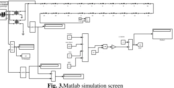
The vehicle power increases with the traction force and vehicle speed. The equivalent circuit given with Figure 1 was simulated with different operating parameters and 1000 data arrays were obtained regarding different operating conditions. The parameters used in the simulation are the number of vehicles, acceleration-mass value of the vehicle, vehicle motion resistance, curve radius, slope, the length of the supply line, internal consumption current of the vehicle, electric resistance and inductance of the line; the calculated value is the highest voltage drop value occurring on the line. Random values were assigned to all the input parameters used in the simulation.

II.

MATERIAL

AND

METHOD

In this study, the artificial neural network, adaptive fuzzy inference system and support vector machine among the artificial intelligence applications were used for the simulation. The ANFIS is a hybrid artificial intelligence method which uses the parallel computing and learning capability of artificial neural networks and the inferential characteristic of fuzzy logic. The ANN is a method which functions by imitating the way of work of a simple biological nervous system. The SVM is one of the quite effective and simple methods used in classification. For classification, it is possible to divide the two groups by drawing a line between two groups on a plane. The location on which this line will be drawn should be the farthest place to the members of both groups. The SVM determines how this line will be drawn. Matlab and Weka program was used for the simulation.

1000 data arrays different from each other were used for the matlab simulation. The simulation were run for 1000 different operation conditions. The matlab simulation screen is given with Figure 3.

Fig. 3.Matlab simulation screen

A. Adaptive Neuro Fuzzy Inference System (ANFIS)

The ANFIS is a class of adaptive networks functionally equivalent to the fuzzy inference system. The ANFIS can be given more integrated with some characteristics of controllers, learning ability, parallel processing, structured knowledge representation, other supervision and design methods. Fuzzy logic and neural networks are supplementary means used together in developing smart systems [13-15]. The ANFIS consists of 6 layers. This system is displayed in Figure 4. The node functions of every layer in the ANFIS structure and the operation of the layers are respectively as follows [15]. First layer is named the input layer. The input signals obtained from every node in this layer are transmitted to other layers. Second layer is named the fuzzification layer. In separating the input values into fuzzy sets, Jang’s ANFIS model uses the Bell activation function generalized as a membership function. Here, the output of each node consists of membership degrees based on the input values and the membership function used and the membership values obtained from the 2nd layer are presented as µ_𝐴

𝑗(𝑥) × and µ𝐵𝑗(𝑦) Third layer is the layer of rules. Each node in this layer expresses the rules

established in accordance with the Sugeno fuzzy logic inference system and their number. The output of each rule node µ_iturns out to be the multiplication of membership degrees which arrive from the 2nd layer. The acquisition of µ_i values, on the condition that (j=1,2) and (i=1,….,n), is as follows:

𝑦𝑖3=П𝑖 =µ_𝐴𝑗(𝑥) ×µ_𝐵𝑗(𝑦) =µ_𝑖 (7)

Here, 𝑦𝑖3 represents the output values of the 3rd layer; n represents the number of nodes in this layer.

Fourth layer is the normalization layer. Each node in this layer regards all the nodes coming from the rule layer as input values and computes the normalized ignition level of each rule. The computing of the normalized ignition level 𝜇 𝑖 is performed in accordance with the following formula:

𝑦𝑖4= 𝑁𝑖=

µ_𝑖 µ_𝑖 𝑛 𝑖=1

=µ_𝑖 (i=1,n) (8)

Fifth layer is the purification layer. The weighted resulting values of a given rule in each node in the purification layer are calculated. The output value of the ith node in the 5th layer is as follows.

𝑦𝑖5=µ_𝑖 𝑝𝑖𝑥1+ 𝑞𝑖𝑥2+ 𝑟𝑖 , (i=1,n) (9)

cer gucu

arac direnci

kurp

egim

ic tuketim

1 2 3 4 5 6 7 8 9 10

20 11 21 22 12 13 14 15 16 17 18 19 powergui Discrete , Ts = 0.0001 s

-C-The (pi , qi , ri ) variables here are the outcome parameter set of the ith rule. Sixth is the sum layer. There is only one node in this layer and it is labeled as Σ.The output value of each node in the 5th layer is summed here so that the actual value of the ANFIS system is obtained. The computing of y, which is the output value of the system, is performed in accordance with the equation below [15].

𝑦 = 𝑛_𝑖=1µ_𝑖 𝑝𝑖𝑥1+ 𝑞𝑖𝑥2+ 𝑟𝑖 (10)

Fig. 4: ANFIS structure

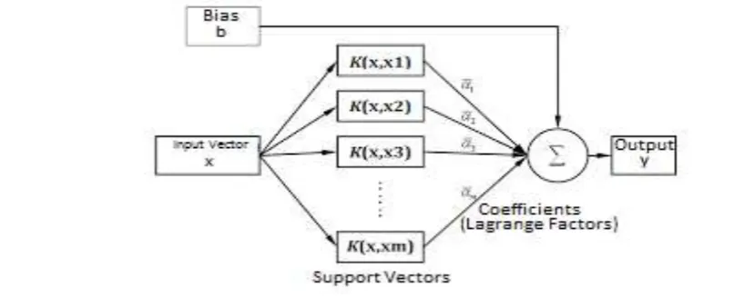
B. Support Vector Machines (SVM)

The Support vector machines can be employed in classification and regression problems. The basic idea in the SVM regression method is finding the linear separator function which reflects the characteristic of the educational data available in a way as closest to reality as possible and suits the statistical learning theory. Similarly to the classification, in the regression, the core functions are used for the non-linear situations to be processed. The most significant advantage of the Support Vector Machines is to solve the classification problem by converting it to a squared optimization problem. This way, at the learning stage regarding the solution of the problem, the number of operations decreases and the solution is reached more rapidly when compared to other techniques/algorithms. The technique, due to this characteristic of it, provides a great advantage, especially in bulky data sets. Furthermore, since it is optimization-based, it is more successful in terms of the classification performance, computational complexity and practicality when compared to other techniques [16-19].

A support vector machine constitutes an n-dimensional hyperplane which optimally divides the data into two categories. The SVM models are closely related to the artificial neural networks and the SVM, which uses a sigmoid kernel function, has a two-layer, feed-forward artificial neural network. The interesting characteristic of the SVM is that it functions with the quality of structural risk minimization in the statistical learning theory rather than the empirical risk minimization principle derived by minimizing the mean squared error on the data set. One of the basic assumptions of the SVM is the independent and similar distribution of all samples in the education set. The SVM can be employed in classification and regression problems. The basic idea in the SVM regression method is finding the linear separator function which reflects the characteristic of the educational data available in a way as closest to reality as possible and suits the statistical learning theory. Similarly to the classification, in the regression, the core functions are used for the non-linear situations to be processed. Two situations that can be encountered in the Support Vector Machines are the data’s being of a structure that can be linearly separated or cannot be linearly separated. The SVM network structure is given with Figure 5.

Fig. 5: Support vector machine structure

A

1

A

2

B

1

B

2

Π

1

Π

2

Π

3

Π

4

1

N

1

N

2

N

3

N

4

Σ

2

3

4

y

x1

x2

2.

Layer

2.

Katma

n

3.

Layer

3.

Katma

n

4.

Layer

4.

Katma

n

5.

Layer

5.

Katma

n

6.

Layer

6.

Katma

n

x1 x2

The Support Vector Machine (SVM) is a controlled classification algorithm based on the statistical learning theory. The mathematical algorithms that the SVM has were initially designed for the classification problem of two-class linear data but later they were generalized for the classification of multi-class and non-linear data.

The SVM regression uses a set of core functions for simulations. In this study, the normalized polynomial kernel was selected and is given by equation (11) and (12).

K(x, y) =< 𝑥, 𝑦 >÷ (< 𝑥, 𝑥 >< 𝑦, 𝑦 >)(11)

< 𝑥, 𝑦 >= 𝑃𝑜𝑙𝑦𝐾𝑒𝑟𝑛𝑒𝑙(𝑥, 𝑦) (12)

C. Artificial Neural Networks (ANN)

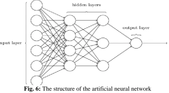
Artificial neural networks emerged as a mathematical method from the latest outputs of endeavors to study and imitate human nature. Artificial neural networks take computing and data processing power from their parallel distributed structure, their capability to learn and generalize. Generalisation is defined as artificial neural networks’ producing proper reactions to the inputs which have not been experienced in the course of education or learning. These characteristics indicate the problem-solving capability of artificial neural networks [20-25]. The biological neuron consists of a nucleus, body and two extensions. The structure of the artificial neural network is given in Figure 6. The 1st layer is the input layer. Data are received from here and entered into the system. The 2nd layer is the hidden layer. Its use depends on the simulation. The 3rd layer is the output layer. Inputs are processed and received from here. Each sphere (nerve) has a function and a threshold value. Filled small circles indicate bonding weights [26-30].

Fig. 6: The structure of the artificial neural network

The output of a neuron is given with (13) as a function formed by adding a bias value to the sum of the input data in specific weights. “I”s indicate the input, “W”s are the coefficients that the input values take.

𝑂𝑢𝑡𝑝𝑢𝑡 = 𝑓(𝑖1𝑊1+ 𝑖2𝑊2+ 𝑖3𝑊3+ 𝑏𝑖𝑎𝑠)(13)

III.

FINDINGS

1000 data arrays different from each other were used for the calculation of the voltage drop created by the traction force. A portion of the data used is displayed in Table 1.

Table 1:A portion of the data set that used

Inputs Output

Number of Vehicles

Ma Val ue (kN )

Vehicle Motion Resistanc

e (kN)

Curve Radius (m)

Slope Voltage Drop

(V)

Internal Consumption

Current of the Vehicle

(A)

Line Resistance

(Ω)

Line Inductan

ce (L)

The Length

of the Supply

Line (km)

A. Simulation Results With the ANFIS

The structure of the system created for the ANFIS and the simulation results are given below. A structure with 9 inputs 2 membership functions created for the ANFIS is given with Figure 7. A triangular-shaped membership function was used for the simulation.

Fig. 7: Triangular-shaped membership function

29 = 512 rules were established for the ANFIS design. The ANFIS architecture is shown in Figure 8. The system consists of the input, input MF, Rule, output MF and output modules.

Fig. 8: ANFIS architecture

The realized data and the data calculated by the ANFIS are shown in Figure 9. The output values are shown with (o) and prediction values are shown with (*).

The realized values and calculated values of all data are shown with the ANFIS simulation with Figure 9. The regression value for all data is 0.63.

Fig. 9: ANFIS regression graph

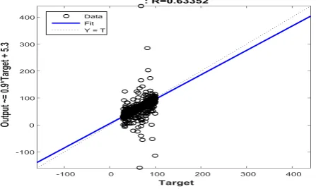
B. Simulation Results With the SVM

By trying different variations to obtain better results in the simulation, the SVM parameters were eventually selected as follows. The complexity parameter “c=1” was selected. The normalized polynomial kernel function was selected as the core function and the exponent value was taken as “e=3”. Test mode 10-fold cross-validation was selected in WEKA.

The realized values and calculated values of all the data are observed in figure 10. The regression value is shown with R and as seen in the figure, this value is 0,92.

input

output

Fig. 10: SVM regression graph

C. Simulation Results With the ANN

As seen in Table 1, the system consists of 9 input and 1 output parameters. The ANN architecture used is given in Figure 11.

Fig. 11: ANN architecture designed [MATLAB R2015b]

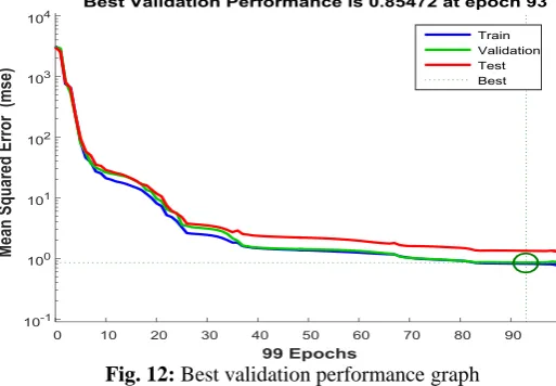
9 input data, 10 hidden neurons, 1 output neuron and 1 output data were used for the ANN architecture used in the design. 70% of the data used for simulation were used for education, 15% for validation, 15% for the test. As seen in Figure 12, the best validation value was reached at the 93th iteration by inhibiting overfitting in the simulation. The lowest mean squared error value is 0.85472. The training, validation and test data produced by the system displayed similar characteristics. Since the validation error value increased in the course of 6 iterations, the simulation was stopped at the end of 99 iterations.

Fig. 12: Best validation performance graph

6 iterations. The mse performance is given with the training state graph. Gradient=27.6801 at epoch 99, mu=0.0001 at epoch 99 and the validation checks=6 at epoch 99.

Fig. 13: Training state graph

The error histogram is shown in Figure 14. The differences between the realized values and calculated values are seen with this graph. The distribution of the errors of the training data is shown with blue, validation data with green and test data with red. The errors mostly concentrate between -1.75 and 2.549.

Fig. 14: Error histogram

The realized and calculated values of the training, validation and test data are seen in Figure 15. The regression value is shown with R, and as seen in the Figure 9, these values are 0.99909 for training, 0.99896 for validation, 0.99840 for the test data. The R value is 0.99897 for all data. As this value approaches 1, the accuracy of the data calculated by the system increases.

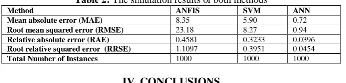
D. The Comparison of the ANFIS, SVM and ANN Results

When the ANN, SVM and ANFIS results are compared, the ANN results are observed to be better. The simulation results of both methods are given in Table 2.

Table 2: The simulation results of both methods

Method ANFIS SVM ANN

Mean absolute error (MAE) 8.35 5.90 0.72

Root mean squared error (RMSE) 23.18 8.27 0.94

Relative absolute error (RAE) 0.4581 0.3233 0.0396

Root relative squared error (RRSE) 1.1097 0.3951 0.0454

Total Number of Instances 1000 1000 1000

IV.

CONCLUSIONS

In this study, the prediction of the distance between AC traction power centerson an AC supplied railway with regard to the operating data was performed. 1000 random input data arrays and the calculated output data were used for the simulation. In the analyses carried out, the ANFIS, SVM and ANN techniques were used. The distance value was predicted. The RRSE value in the data obtained for the ANFIS in the calculations carried out is 111% , this value is 40% in the SVM and 4% in the ANN. The RMSE values are 23 V for the ANFIS simulation, 8 V for the SVM and 1 V for the ANN. The MAE value acquired in the ANFIS is 8 V, in the SVM is 6 V, this value is 1 V in the ANN. The RAE value in the ANFIS is 46%, in the SVM is 32%, this value is 4% in the ANN. When the data obtained from the simulations are compared, the prediction values produced with the ANN are observed to be better. When the prediction data produced for both techniques are compared with the real data, it is observed that errors are at an acceptable rate and that the prediction data produced are usable.

REFERENCES

[1]. Huh JS, Shin HS, Moon WS, Kang BW, Kim JC. Study on voltage unbalance improvement using SFCL in power feed network with electric railway system. IEEE Transactions on Applied Superconductivity 2013; 3: 3601004.

[2]. Ghassemi A, Fazel SS, Maghsoud I, Farshad S. Comprehensive study on the power rating of a railway power conditioner using thyristor switched capacitor. IET Electrical Systems in Transportation 2014; 4: 97-106.

[3]. Raimondo G, Ladoux P, Lowinsky A, Caron H, Marino P. Reactive power compensation in railways based on AC boost choppers. IET Electrical Systems in Transportation 2012; 2: 169-177.

[4]. Aodsup K, Kulworawanichpong T. Effect of train headway on voltage collapses in high-speed AC railways. In: APPEEC 2012 Power and Energy Engineering Conference; 27-29 March 2012; Shanghai, China. New York, USA: IEEE. pp. 1-4.

[5]. Baseri MAA, Nezhad MN, Sandidzadeh MA. Compensating procedures for power quality amplification of AC electrified railway systems using FACTS. In: PEDSTC 2011 Power Electronics Drive Systems and Technologies Conference; 16-17 Februrary 2011; Tehran, Iran. New York, USA: IEEE. pp. 518-521. [6]. Brenna M, Foiadelli F. The compatibility between DC and AC supply of the Italian railway system. In:

Power and Energy Society General Meeting; 24-29 July 2011; San Diego, USA. New York, USA: IEEE. pp. 1-7.

[7]. Abrahamsson L, Kjellqvist T, Ostlund S. High-voltage DC-feeder solution for electric railways. IET Power Electronics 2012; 5: 1776 - 1784.

[8]. Raygani SV, Tahavorgar A, Fazel SS, Moaveni B. Load flow analysis and future development study for an AC electric railway. IET Electrical Systems in Transportation 2012; 2: 139-147.

[9]. Goodman CJ, Chymera M. Modelling and simulation. In: REIS 2013 Railway Electrification Infrastructure and Systems Conference; 3-6 June 2013; London, England. New York, USA: IEEE. pp. 16-25.

[10]. Ladoux P, Raimondo G, Caron H, Marino P. Chopper-Controlled steinmetz circuit for voltage balancing in railway substations. IEEE Transactions on Power Electronics 2013; 28: 5813-5822.

[11]. Shin, HS, Cho SM, Kim JC. Protection scheme using SFCL for electric railways with automatic power changeover switch system. IEEE Transactions on Applied Superconductivity 2012; 20: 5600604.

[12]. Shin HS, Cho SM, Huh JS, Kim, JC, Kweon, DJ. Application on of SFCL in automatic power changeover switch system of electric railways. IEEE Transactions on Applied Superconductivity 2012; 22: 5600704. [13]. Ozkan IA, Saritas I, Herdem S. Modeling of magnetic filtering with ANFIS. In: 12. National Conference

[14]. Sit S, Ozcalik HR, Kilic E, Dogmus O, Altun M. Investigation of performance based on online adaptive neuro-fuzzy ınference system (ANFIS) for speed control of ınduction motors. Cukurova University Journal of the Faculty of Engineering and Architecture 2016; 31: 33-42.

[15]. Jang, JSR. ANFIS: Adaptive-network-based fuzzy inference system. IEEE Transactions on Systems, Man, and Cybernetics 1993; 23: 665–685.

[16]. Ayhan, S., Erdogmus, S. Kernel function selection for the solution of classification problems via support vector machines, Eskisehir Osmangazi University Journal Of IIBF, 9, 175-198, 2014.

[17]. Yakut, E., Elmas, B., Yavuz, S. Predictıng stock-exchange index using methods of neural networks and support vector machines, SuleymanDemirel University The Journal Of Faculty Of Economics And Administrative Sciences, 19, 139-157, 2014.

[18]. Kavzaoglu, T., Colkesen, I. Investigation of the effects of kernel functions in satellite image classification using support vector machines, Gebze High Technology Institute The Journal of Map, 144, 73-82, 2010. [19]. Guran, A., Uysal, M., Dogrusoz, O. Effects of support vector machines parameter optimization on

sentiment analysis, DEU Engineering Faculty The Journal Of Engineering Sciences, 16, 86-93, 2014. [20]. Ozdemir H. Artificial neural networks and their usage in weaving technology. Electronic Journal of Textile

Technologies 2013; 7: 51-68.

[21]. Sahin M, Buyuktumturk F, Oguz Y. Light quality control with artificial neural networks. AfyonKocatepe University Journal of Science and Engineering 2013; 13: 1-10.

[22]. Bayindir R, Sesveren Ö. Design of a visual interface for ANN based systems. Pamukkale University Engineering Faculty Journal of Engineering Science 2008; 14: 101-109.

[23]. Askin D, Iskender I, Mamızadeh A. Dry type transformer winding thermal analysis usıng different neural network methods. Journal of the Faculty of Engineering and Architecture of Gazi University 2011; 26: 905-913.

[24]. Cavuslu MA, Becerikli Y, Karakuzu C. Hardware implementation of neural network training with levenberg-marquardt algorithm. Journal of Computer Science and Engineering 2012; 5: 31-38.

[25]. Dalkiran İ, Danisman K. Artificial neural network based chaotic generator for cryptology. Turkish Journal Of Electrical Engineering And Computer Sciences 2010; 18: 225-240.

[26]. Ceylan M, Ozbay Y, Ucan ON, Yildirim E. A novel method for lung segmentation on chest ct images: complex-valued artificial neural network with complex wavelet transform. Turkish Journal Of Electrical Engineering And Computer Sciences 2010; 18: 613-623.

[27]. Partal S, Senol İ, Bakan AF, Bekiroglu KN. Online speed control of a brushless AC servomotor based on artificial neural networks. Turkish Journal Of Electrical Engineering And Computer Sciences.2011; 19: 373-383.

[28]. Jashfar S, Esmaeili S, Jahromi MZ, Rahmanian M. Classification of power quality disturbances using s-transform and tt-s-transform based on the artificial neural network. Turkish Journal Of Electrical Engineering And Computer Sciences. 2013; 21: 1528-1538.

[29]. Afsharizadeh M, Mohammadi M. Prediction-Based reversible ımage watermarking using artificial neural networks. Turkish Journal Of Electrical Engineering And Computer Sciences 2016; 24: 896-910.

[30]. Minaz MR, Gun A, Kurban M, Imal N. Estimation of pressure, temperature and wind speed of bilecik using different methods. Gaziosmanpasa Journal of Scientific Research 2013; 3: 100-111.