TA Hybrid Conjoint Analysis (CA)-CBR Parameterization Module for Genetic Algorithm in Project Scheduling

(1)

ISSN (Online) 2249-6084 (Print) 2250-1029 www.eijppr.com

A Hybrid Conjoint Analysis (CA)-CBR

Parameterization Module for Genetic Algorithm in

Project Scheduling

Mahdi Sharifmousavi

1

_{, Jamal Shahrabi}

2

_*

1_{PhD Candidate of Industrial Engineering-Industrial Engineering and Management Systems Department, AmriKabir} University of Technology (AUT),

2_{Assistant Professor-Industrial Engineering and Management Systems Department, AmriKabir University of} Technology (AUT).

ABSTRACT

Resource Constrained Project Scheduling Problem (RCPSP) is a classical, well studied OR problem. Because of its NP-Hard nature, it is well suited to meta-heuristic (MH) algorithms; the performance of these algorithms are highly dependent on their initial parameters values, but this issue is ignored in most MH implementations, and only few researches have been performed in this area. This article offers a contribution to address this shortcoming using Conjoint Analysis (CA) and Case Based Reasoning (CBR). At first, different approaches to code RCPSP problem for Genetic Algorithm (GA) are explored, and then a novel full profile CA approach is used to propose parameterization schemes for sample projects to form initial case base; after forming the initial case base, Case Based Reasoning (CBR) is used to propose parameterization schemes for new projects. A Multivariate Data Analysis (MDA) model is devised to determine the near optimal parameterization scheme for RCPSP. The performance of the proposed model is compared with GA algorithm with average parameterization scheme and Tabu Search (TS) algorithm. The results show the superiority of this approach to random parameterization of GA algorithm.

Key Words: Resource Constrained Project Scheduling Problem (RCPSP), Conjoint Analysis (CA), Case Based Reasoning (CBR), Genetic Algorithm (GA).

eIJPPR 2018; 8(4):70-83 HOW TO CITE THIS ARTICLE: Mahdi Sharifmousavi1, Jamal Shahrabi(2018). “A hybrid conjoint analysis (CA)-CBR parameterization module for genetic algorithm in project scheduling”, International Journal of Pharmaceutical and Phytopharmacological Research, 8(4), pp.70-83.

INTRODUCTION

Resource Constrained Project Scheduling Problem (RCPSP) has been a research topic for many decades, and several optimization schemes have been used to solve this problem [1]. RCPSP aims at minimizing the total duration of the project subject to two types of constraints: precedence and resource constraints. Precedence relationships force some activities to begin after the finalization of others. In addition to precedence constraints, every activity requires a predefined amount of resources. There are different types of resources identified in the literature based on different perspectives, including renewable, non-renewable, and doubly constrained

resources [2]. RCPSP considers resources of limited availability and activities of known durations and resource requests, linked by precedence relations. The problem consists of finding a schedule of minimal duration by assigning a start time to each activity such that the precedence relations and the resource availabilities are respected.

According to the computational complexity theory [3], RCPSP belongs to the class of problems that are NP-hard in the strong sense [4-6]. There is a broad spectrum of methods used to solve RCPSP. Detailed history of methods used to solve RCPSP is described in [7, 8]. According to NP-Hard complexity of RCPSP, researchers believe that optimal solution can be achieved by exact procedures only in small projects, usually with less than

Corresponding author: Jamal Shahrabi

Address: Assistant Professor-Industrial Engineering and Management Systems Department, AmriKabir University of Technology (AUT).

E-mail: jamalshahrabi @ aut.ac.ir

Relevant conflicts of interest/financial disclosures: The authors declare that the research was conducted in the absence of any commercial or financial relationships that could be construed as a potential conflict of interest .

(2)

71

60 activities [9] and less than two renewable resources [10]. An overview of deterministic, heuristic, and meta-heuristic methods used to solve RCPSP is illustrated in Table 1. The focus is more on meta-heuristics.

Table 1: Overview of algorithms used to solve RCPSP

row

Reference number

Deterministic Heuristic Meta-heuristic

L ine ar P rogra m m ing T ree s ear ch 0 -1 Int eg er prog ra m m ing M ixe d i n te ge r pr ogra m m ing L ist -ba se d ne igh borhoods S et ba se d ne ighb ors ext end ed n ei ghb orhood for na tura l da te va ri abl es S im ul at ed A nne al ing T ab u S ear ch A nt Col ony O pt im iz at ion G en eti c A lg o rith m

1 (Slowinski 1980) [11] *

2 (Patterson 1984) [12] *

3 (Mingozzi et al.

1998) [13] *

4

(RAMLOGAN and GOULTER

1989) [14]

*

5 (Fleszar and

Hindi 2004) [15] *

6

(Tonius Baar, Brucker, and Knust 1998) [16]

* 7 (Artigues, Michelon, and Reusser 2003) [17] * 8 (Palpant, Artigues, and Michelon 2004) [18] *

9 (BOCTOR

1996) [19] *

10

(Bouleimen and Lecocq 2003)

[20]

**

11 (Thomas and

Salhi 1998) [21] **

12 (Debels et al.

2006) [22] * **

13 (Merkle, Middendorf, and Schmeck 2002) [23] * ** 14 (Kochetov and Stolyar 2003) [24] **

15 (Mori and Tseng

1997) [25] * *

16 (Ozdamar 1999)

[26] * *

17 (Sonke Hartmann 2001) [27] * * 18 (Kohlmorgen, Schmeck, and Haase 1999) [28] * 19 (Alcaraz and Maroto 2001) [9] *

20 (Lova et al.

2009) [29] *

21 (Zoulfaghari et

al. 2013) [30] *

Heuristic procedures seek acceptable solutions with few computational requirements, instead of necessarily optimal solution. Heuristic and meta-heuristic procedures are suitable for large projects with large number of resources. These procedures are divided into construction and improvement heuristics [31]; construction heuristics are used to generate a first solution in a reasonable amount of time. Improvement heuristics are used to improve constructed solutions.

Meta-heuristics aim at dealing with the main problems of heuristic methods including their problem specific nature and shortcomings in escaping from local optima and exploring neighbors. Most meta-heuristics include stochastic components [32]. [8] shows that meta-heuristics outperform heuristic algorithms in RCPSP. Several meta-heuristic algorithms have been used to solve RCPSP. Simulated annealing belongs to improvement heuristics, and the method attempts to simulate the way metals cool and anneal [33]. [8, 19, 20] used simulated annealing to solve RCPSP. Tabu search is another meta-heuristic algorithm that tolerates non-improving moves in the neighbor. A short term memory of recent moves or solutions called Tabu list is used to prevent cycling. Some of the most important researches that use Tabu search for RCPSP are [16, 21, 22]. Evolutionary approaches are the most popular heuristic approach for RCPSP. In these approaches, population of solutions evolves according to specific algorithm [34]. [23] used ant colony optimization together with local search to solve RCPSP. [24] proposed a hybrid evolutionary method based on path relinking, Grasp and Tabu search. Genetic algorithm is the most popular optimization scheme for RCPSP in recent years and has been proposed by [9, 25-30, 35, 36].

Comparing the numerical results of some of these researches, genetic algorithm used by [9] outperformed simulated annealing used by [20] and genetic algorithm proposed by [36]; this is because of different representation schemes used, natural date variables for [36], and set-based representation for [9].

(3)

72

retrieve, reuse, revise, and retain. CBR related method was also successfully used for optimization problems and especially combinatorial optimization problems including

TSP [38, 39], knapsack problem[40], and wide range of

scheduling related problems, [41] implying that CBR is an appropriate approach for scheduling problems. Some of the successful applications of CBR in this area are: production planning and control problems [42], dynamic production scheduling [43], meta-heuristic time tabling [44, 45], meta-heuristics runtime estimation [46], and project scheduling [47].

The performance of meta-heuristics is highly dependent on their parameter values initialization. There is no formal process to define parameter values at the start of using meta-heuristics, and the parameter values are highly dependent on problem nature itself. There are few efforts performed to develop formal models for initial parameterization in the area of combinatorial problems, especially scheduling related problems. one of the major efforts in this area is development of self-optimization module that can propose meta-heuristic algorithm and its parameterization scheme for dynamic scheduling problem using case based reasoning [41, 43]. Those articles depend on randomly suggesting parameterization schemes for some projects to develop initial case base and then proposing parameterization scheme based on similarity between new project and projects stored in case base. They provide no rule for developing dependable case base.

Conjoint Analysis (CA) is a multivariate data analysis (MDA) and data mining technique used to clarify how respondents develop preferences for products and services [48]. The dependent variable is a measure of respondents’ preferences and can be metric or non-metric. The independent variables are dummy variables representing attributes of multi-attribute products or services; these preferences are the inputs for market simulation techniques [49]. CA has been used in many areas including food industry [50], psychology [51], healthcare [52], supply chain management [53], and operations management [54].

This is the first study that uses CA to address the MH algorithms parameterization issue; CA has been used to find the optimal parameterization scheme for MH algorithms in RCPSP resolution; according to the popularity of using GA for RCPSP resolution, MH algorithm was used for the study. After forming initial case base with CA, CBR was used to propose parameterization scheme for new projects. The rest of the article is organized as follows: section 2 describes the RCPSP formulation as optimization problem and coding of this problem to solve by MH algorithm; section 3 describes the CA algorithm and CBR; section 4 evaluates

the performance of proposed Conjoint Based CBR algorithm.

RCPSP

RCPSP can be defined as a combinatorial optimization problem. A combinatorial optimization problem is defined by a solution space X, which is discrete or can be reduced to a discrete set by a subset of feasible solutions

𝑌𝑌 ⊆ 𝑋𝑋 associated with an objective function𝑓𝑓:𝑌𝑌 → 𝑅𝑅. A combinatorial optimization problem aims at finding a

feasible solution y ∈ Y such that f(y) is minimized or

maximized. A resource-constrained project scheduling problem is a combinatorial optimization problem defined by a tuple (V, p, E, R, B, b) [34] in which this tuple members are representing activity set, duration set, resource set, availability of resources set, and required resources by activity set, respectively. Equation 1 shows the RCPSP as an optimization problem. The make span of

schedule S is equal to 𝑆𝑆_𝑛𝑛+1 which is the startup of end

activity (activities 0 and n+1 are fictitious activities

representing start and end of the project); 𝑝𝑝_𝑖𝑖 represents

the duration of activity; 𝐴𝐴𝑖𝑖 𝑏𝑏𝑖𝑖𝑖𝑖 represents the amount of

resource 𝑅𝑅𝑖𝑖 used per time during the execution of

activity; 𝐴𝐴𝑖𝑖 and 𝐵𝐵𝑖𝑖 denotes the availability of 𝑅𝑅𝑖𝑖.

Equation 1: Formulation of RCPSP as an integer programming problem

Resource Constrained Project Scheduling Problem(Project Duration Minimization)

Objective

Function: 𝑚𝑚𝑚𝑚𝑚𝑚:𝑆𝑆𝑛𝑛+1

Constraints: 𝑆𝑆_𝑗𝑗− 𝑆𝑆_𝑖𝑖 ∀(A_𝑖𝑖,A_j)∈𝐸𝐸

� 𝑏𝑏𝑖𝑖𝑖𝑖≤ 𝐵𝐵𝐾𝐾 𝐴𝐴𝑖𝑖∈𝐴𝐴𝑡𝑡

∀R_K∈R , ∀ t≥0

RCPSP Coding (Schedule Generation Scheme)

(4)

73

and serial SGS deliver better results compared to other representation schemes of RCPSP. According to the findings, serial SGS is used for coding. For representing each project, using GA, each chromosome is as long as the number of project activities, and each gene is a random number between 0 and 1. By sorting the genes of each chromosome and replacing each gene number with its rank, a rough schedule is generated. This schedule is repaired according to precedence constraints. Figure 1 shows a sample project; these processes are shown in

Figure 2; this feasible schedule is used to develop the final schedule according to resource constraints.

0

1

2

3

4

5 6 7

8 9 10 11

12

13 14 end

Fig. 1: Sample project network

Fig. 2:Network generation scheme

Genetic Algorithm Implementation on RCPSP

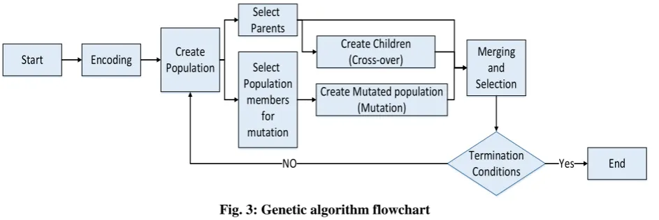
In RCPSP like other engineering problems, genetic algorithm includes encoding, selection, cross-over, mutation, substitution, and iteration operations. Considering these operations within chronological order, the final stages are:

• Encoding

• Creating random population and evaluation

• Selecting parents and using them to create

children (cross-over)

• Selecting population members for mutation and

creating mutated population

• Combining parent, cross-over and mutated

population and creating new population

These stages are illustrated in Figure 3. The main issues that should be considered in practicing genetic algorithm are: 1. exploration and exploitation ability; 2. convergence and diversity of population, and 3. the nature of different RCPSPs. One of the most important issues in this part is the feasibility of each solution that are guaranteed using the repair mechanism after generation of different random schedules. There are different termination rules for genetic algorithm like any meta-heuristic algorithm including: reaching acceptable value, certain amount of iterations, computation time, the number of function evaluations, and stalled iterations [56].

Start

Select Parents Create

Population

Encoding _Select

Population members

for mutation

Create Children (Cross-over)

Create Mutated population (Mutation)

Merging and Selection

Termination Conditions

NO Yes End

(5)

74

The main areas adjusted in GA to find the best or acceptably good parameterization scheme are:

1. Selecting parents

2. Combining parents (cross-over mechanisms)

3. Selecting population members for mutation

4. Mutation

5. Selecting new population

Detailed programming of these items will be discussed in the following sections.

Selection

The first population is created by generating random numbers for each gen and then sorting the gens and repairing random schedule generated. There are different parent selection methods used in this study: roulette wheel selection [57], tournament selection [58], and random selection of one of these two methods. In roulette wheel selection, selection is based on random number generation and probability values. In tournament selection, samples with ‘m’ members were selected from the population, and the best member of this sample was selected as a parent; in this method, the worst m-1 members of the population have no chance to be selected as a parent. In roulette wheel selection, selection is based on discrete statistical distribution; a good example is Boltzmann method (Equation 2) [59]:

Equation 2

𝑝𝑝𝑖𝑖∝ 𝑒𝑒−𝑐𝑐𝑖𝑖

The probabilities can be altered using selection pressure parameter (β); by imposing selection pressure to probabilities, the environment can be changed. New

probabilities (𝑝𝑝𝑖𝑖) are calculated using Equation 3:

Equation 3

𝑝𝑝𝑖𝑖=_∑(𝒑𝒑𝒊𝒊₍_𝒑𝒑′)𝜷𝜷

𝒋𝒋 ′₎𝜷𝜷 𝒋𝒋

If β=0, the fine selection becomes the uniform random selection, and if β→∞, only the member with the greatest

value of 𝒑𝒑_𝒊𝒊′ is selected. If β is imposed to Boltzmann

method, the final value of probabilities is calculated using Equation 4.

Equation 4

𝑝𝑝𝑖𝑖= 𝒆𝒆−𝜷𝜷𝒄𝒄𝒊𝒊

∑ 𝒆𝒆−𝜷𝜷𝒄𝒄𝒋𝒋

𝒋𝒋

Crossover

Based on the type of coding (binary or continuous), different operations have been used for cross-over. Within binary problems, single and double point cross overs are more popular. In single point cross-over, two chromosomes are cut at the same point, and their parts are shifted and create two child chromosomes; in double

point cross-over, there are two cutting points, and the central part of two chromosomes are replaced and create two child chromosomes. The other method for discrete environments is uniform cross-over [60]; in this method,

the child chromosomes, 𝑦𝑦1𝑖𝑖and 𝑦𝑦2𝑖𝑖, are calculated using

Equation 5. This method has more exploration ability in comparison with previous methods.

Equation 5

𝑦𝑦1𝑖𝑖=∝𝑖𝑖𝑥𝑥1𝑖𝑖+ (1−∝𝑖𝑖)𝑥𝑥2𝑖𝑖 𝑦𝑦2𝑖𝑖=∝𝑖𝑖𝑥𝑥2𝑖𝑖+ (1−∝𝑖𝑖)𝑥𝑥1𝑖𝑖

∝𝑖𝑖∈{0,1}

In this problem, because of its continuous nature, each

gene is a real number in the range of [𝑥𝑥𝑚𝑚𝑖𝑖𝑛𝑛,𝑥𝑥𝑚𝑚𝑚𝑚𝑚𝑚]. The

above mentioned methods are not applicable, so the Arithmetic cross-over is used; this method is similar to

uniform cross-over unless 0≤∝𝑖𝑖≤1. In order to

strengthen the exploration ability of the algorithm and cover the areas outside the range of two parents, the

parameter gamma and −𝛾𝛾 ≤∝𝑖𝑖≤1 +𝛾𝛾 were used.

Mutation

In mutation, the intensity of changes must be determined.

For this purpose, the mutation influence factor (0≤

𝜋𝜋𝑚𝑚≤1) was used (Equation 6); if 𝜋𝜋𝑚𝑚= 1, all genes will

undergo mutation, and if 𝜋𝜋𝑚𝑚= 0, no mutation will be

performed on the chromosome.

Equation 6

𝑁𝑁𝑁𝑁𝑚𝑚𝑏𝑏𝑒𝑒𝑁𝑁𝑜𝑜𝑓𝑓𝑚𝑚𝑁𝑁𝑚𝑚𝑚𝑚𝑚𝑚𝑒𝑒𝑚𝑚𝑔𝑔𝑒𝑒𝑚𝑚𝑒𝑒𝑔𝑔=𝜋𝜋𝑚𝑚.𝑚𝑚𝑣𝑣𝑚𝑚𝑣𝑣

In binary problems, the only thing which has to be done is changing the genes values from 0 to 1 or 1 to 0; in integer problems, the genes only have to change to other integer numbers. In real problems, the gene value could be any number within the defined range and selected randomly

[61]. Creating new population

There are three different population generation methods during running GA. The first one is merge, sort and truncate, predefined share of parents, children (cross-over) and mutated ones, merge and select randomly, and performing mutation only on offspring generated members. In this study, these methods are used randomly to create new population.

CONJOINT ANALYSIS

(6)

75

clarify how respondents develop preferences for products and services [48]. The dependent variable is a measure of respondents’ preferences and can be metric or non-metric; the independent variables are dummy variables representing attributes of multi-attribute products or services; these preferences are the inputs for market simulation techniques [49]. CA has been used in many areas including food industry [50], psychology [51], healthcare [52], supply chain management [53], and operations management. In this article, parameters of genetic algorithm become the attributes of CA.

The main parameters of CA are: 𝑚𝑚: total number of cards

(combinations of parameters values); 𝑝𝑝: total number of

factors (GA parameters); 𝑚𝑚: total number of discrete

factors; 𝑙𝑙: total number of linear factors; 𝑞𝑞: total number

of quadratic factors; 𝑚𝑚_𝑖𝑖: the number of levels for ith

discrete factor; 𝑚𝑚𝑖𝑖𝑗𝑗 the jth_{level of ith discrete factor;}

1, 2,..., ,

i= d 𝑥𝑥𝑖𝑖: _{the i}th_{linear factor;}_{𝑧𝑧𝑖𝑖}_:_{the i}th_{ideal or}

anti-ideal factor; 𝑁𝑁𝑖𝑖: the ith_{ideal or anti-ideal factor, and}_𝑚𝑚_:_the

total number of subjects analyzed at the same time. The

response 𝑁𝑁_𝑖𝑖 for the ith_{card (product) is calculated using}

Equation 7. 𝑁𝑁_{𝑗𝑗𝑖𝑖}_{𝑗𝑗𝑖𝑖} is the utility (part worth) associated with

the k_jith_{level of j}th_{factor on the i}th_card.

Equation 7

ri=β0+�ujkji

p

j=1

Design matrix is another important part of CA; there is a row for each card (parameter values combination) in the plan file, and the columns of this matrix are defined by each factor variable which can be discrete or linear; the

first column is used to estimate 𝛽𝛽0∗; for discrete factors

with 𝑚𝑚𝑖𝑖 levels, 𝑚𝑚𝑖𝑖−1 columns are formed, each

representing the deviation of one of the factors from the overall mean. The values of 1, a-1, and 0 are inserted in the column if the observed level is overall mean, last level of factor, or otherwise, respectively. These columns are

used to estimate the value of 𝛼𝛼𝑖𝑖𝑗𝑗. For linear factors, there

is a column for each factor which is the centered

(normalized) value of that factor (𝑥𝑥𝑖𝑖𝑗𝑗− 𝑥𝑥𝑖𝑖) used to

estimate 𝑏𝑏𝚤𝚤�. For each quadratic factor, there are two

columns: one with centered (normalized) value of factor (𝑧𝑧𝑖𝑖𝑗𝑗− 𝑧𝑧𝑖𝑖) and the other is the square of the centered

(normalized) value of the factor (𝑧𝑧𝑖𝑖𝑗𝑗− 𝑧𝑧̂𝑖𝑖)2. These two

columns are used to estimate the values of 𝛾𝛾�.

Observations are represented by score or converted to ranks. The general formula for estimates is illustrated in Equation 8. These estimates are calculated using QR

decomposition method. 𝑦𝑦 represents ranks/scores of the

cards and calculated using Equation 9. The

variance-covariance matrix of the above mentioned estimates is illustrated in Equations 10 and 11.

Equation 8

(𝛽𝛽̂𝑖𝑖∗𝛼𝛼�𝛽𝛽̂𝛾𝛾�∗₎′_{= (}_𝑋𝑋′_𝑋𝑋₎−1_𝑋𝑋′_𝑦𝑦

Equation 9

𝑦𝑦𝑖𝑖=�𝑁𝑁_𝑚𝑚𝑖𝑖 _{+ 1}_{− 𝑁𝑁} 𝑚𝑚𝑓𝑓𝑁𝑁𝑒𝑒𝑔𝑔𝑝𝑝𝑜𝑜𝑚𝑚𝑔𝑔𝑒𝑒𝑔𝑔𝑚𝑚𝑁𝑁𝑒𝑒𝑔𝑔𝑠𝑠𝑜𝑜𝑁𝑁𝑒𝑒𝑔𝑔 𝑖𝑖 𝑚𝑚𝑓𝑓𝑁𝑁𝑒𝑒𝑔𝑔𝑝𝑝𝑜𝑜𝑚𝑚𝑔𝑔𝑒𝑒𝑔𝑔𝑚𝑚𝑁𝑁𝑒𝑒𝑁𝑁𝑚𝑚𝑚𝑚𝑟𝑟𝑔𝑔

Equation 10

𝜎𝜎�2₍_𝑋𝑋′_𝑋𝑋₎−1

Equation 11

𝜎𝜎�2₌_{� ��𝑁𝑁𝑖𝑖𝑗𝑗}_{− 𝑁𝑁̂}_{𝑖𝑖𝑗𝑗�}2_/(_{𝑚𝑚𝑚𝑚 − 𝑚𝑚 − 𝑙𝑙 −}₂_{𝑞𝑞 −}₁₎ 𝑛𝑛

𝑗𝑗=1 𝑡𝑡

𝑖𝑖=1

The value of 𝛾𝛾� is calculated using Equation 12 and

Equation 13.

Equation 12

𝛾𝛾�𝑖𝑖1=𝛾𝛾�𝑖𝑖1∗ ₋₂_{𝛾𝛾�𝑖𝑖2}∗ _{∗ 𝑧𝑧̅𝑖𝑖}

Equation 13

𝛾𝛾�𝑖𝑖2=𝛾𝛾�𝑖𝑖2∗

Considering these equations, utility values for different factor levels including discrete, linear, and ideal\anti ideal factors are calculated using Equations 14 to 16, respectively.

Equation 14

𝑁𝑁�𝑗𝑗𝑖𝑖= ⎩ ⎨

⎧𝑚𝑚�𝑗𝑗𝑖𝑖 𝑓𝑓𝑜𝑜𝑁𝑁𝑟𝑟= 1, … ,𝑚𝑚𝑗𝑗−1 − � 𝑚𝑚�𝑗𝑗𝑖𝑖 𝑓𝑓𝑜𝑜𝑁𝑁𝑟𝑟=𝑚𝑚𝑗𝑗

𝑚𝑚𝑗𝑗−1

𝑗𝑗=1

Equation 15

𝑁𝑁�𝑗𝑗𝑖𝑖=𝛽𝛽̂𝑗𝑗𝑥𝑥𝑖𝑖

Equation 16

𝑁𝑁�𝑗𝑗𝑖𝑖=𝛾𝛾�𝑗𝑗1𝑧𝑧𝑗𝑗𝑖𝑖+𝛾𝛾�𝑗𝑗2𝑧𝑧𝑗𝑗𝑖𝑖2

Importance factor is another important outputs of conjoint analysis which illustrates the effect of each factor on final

quality of solution [62]. The importance factor of factor i

is calculated using Equation 17. 𝑅𝑅𝐴𝐴𝑁𝑁𝑅𝑅𝐸𝐸𝑖𝑖 equals to the

(7)

76

Equation 17

𝐼𝐼𝐼𝐼𝐼𝐼𝑖𝑖= 100_{∑ 𝑅𝑅𝐴𝐴𝑁𝑁𝑅𝑅𝐸𝐸𝑖𝑖}𝑝𝑝𝑅𝑅𝐴𝐴𝑁𝑁𝑅𝑅𝐸𝐸𝑖𝑖 𝑖𝑖=1

There are two remaining issues in implementing CA. The first is predicted score for each factor in the case of forecasting scores for new combinations of parameters values performed using Equation 18; the second is the correlation calculation within this algorithm calculated

between predicted score (𝑁𝑁̂𝑖𝑖) and the observed responses

(𝑁𝑁𝑖𝑖) for Pearson and Kendall correlations [63].

Equation 18

𝑁𝑁̂𝑖𝑖=𝛽𝛽̂0+�u�jkji

p

j=1

For simulation applications of CA, the probability 𝑝𝑝𝑖𝑖

should be assigned to each simulation card i (parameter

values combination). These probabilities are computed

based on predicted score (𝑁𝑁̂_𝑖𝑖) for that combination. The

main probability functions t used in this article for simulation purpose are maximum utility [64], BTL [65], and Logit [66]; these three methods are illustrated in Equation 19, Equation 20, and Equation 21, respectively. Probabilities are averaged across different respondents (runs of meta-heuristic algorithms for each combination) in order to obtain grouped simulation results. For the last two methods of probability calculation (BTL and Logit),

only subjects with positive 𝑁𝑁̂𝑖𝑖 are considered.

Equation 19

𝑝𝑝𝑖𝑖=�1 𝑚𝑚𝑓𝑓𝑁𝑁̂𝑖𝑖= max (𝑁𝑁̂𝑖𝑖)

0 𝑜𝑜𝑚𝑚ℎ𝑒𝑒𝑁𝑁𝑒𝑒𝑚𝑚𝑔𝑔𝑒𝑒

Equation 20

𝑝𝑝𝑖𝑖=_{∑ 𝑁𝑁̂}𝑁𝑁̂𝑖𝑖 𝑗𝑗 𝑗𝑗

Equation 21

𝑝𝑝𝑖𝑖= 𝑒𝑒𝑣𝑣̂𝑖𝑖

∑ 𝑒𝑒_𝑗𝑗 𝑣𝑣̂𝑗𝑗

By summing the par-worth of each parameter level in each card, the total utility of the card can be calculated. Because of the time consuming process of CA, this process has been simulated using CBR; based on CBR, the optimal initial parameterization scheme for new projects was determined by adapting the initial parameterization scheme of the previous known project which is most similar to this new project. The overall process of CBR is described in the following section, and then the empirical results of using CA-CBR modules are presented.

CASE BASED REASONING (CBR)

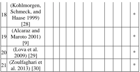
CBR is a promising AI approach for problem solving that suggests new solutions to problems by adapting the most similar old cases’ solutions to the new problem [37]. This approach was inspired by human thinking and behavior. In facing a problem, people search their memory for past experiences with similar situational attributes, they analyze retrieved experiences and apply the learned lessons in these experiences to develop new solutions, and finally, they memorize the problem with success\failure of the final solution for future problems [67]. CBR has four distinct phases known as CBR R4-cycle illustrated in Figure 4 [68]:

1. Retrieve: in this phase, a case-base contains

previously solved problems, and their related solutions are searched, and problems similar to the new problem are retrieved.

2. Reuse: the solutions related to the retrieved cases

are used for solving the new problem through direct using or some combining mechanisms.

3. Revise: the solution resulted from the previous

phase is revised and adapted for solving the new problem.

4. Retain: the new problem and its solution are

(8)

77

Fig. 4: The CBR Cycle [64]

CBR is successfully applied to wide spectrum of applications for various purposes including planning, diagnosis, classification, design, decision making, explanation, and interpretation [69]. CBR related method were also successfully used for optimization problems and especially combinatorial optimization problems including TSP [38, 39], knapsack problem [40], and wide range of scheduling related problems [41], implying that CBR is an appropriate approach for scheduling problems. Some of the successful applications of CBR in this area are: production planning and control problems [69], dynamic production scheduling [43], meta-heuristic time tabling [44, 45], meta-heuristics runtime estimation [46], and project scheduling [47].

In the retrieve phase, the similarity of new project with projects stored in the case base is assessed using parameters presented in Table 2. N is the number of nodes in project Activity on Node (AON) diagram; A is the number of activities (arcs in AON diagram); A’ is the

number of nun-redundant arcs in project diagram; Pi and

Si are the number of predecessors and successors,

respectively. Based on these similarity measures, the two most similar projects stored in the case base were retrieved, and the duration of new project was calculated using both suggested parameterization schemes, and the new project with parameterization scheme with lower duration value was saved in the case base.

Table 2: Case and solution representation

Solution Parameterization schemes

Case related attributes

T-density (- ∑𝑁𝑁_𝑖𝑖=1𝐼𝐼𝑚𝑚𝑥𝑥(0,𝐼𝐼_𝐼𝐼− 𝑆𝑆_𝑖𝑖))-[70] C (A’/N)- [71]

CNC (A/N) [72] Sum of the duration of activities

# of renewable resources # of activities

COMPUTATIONAL RESULTS OF CA-CBR

PARAMETERIZATION MODULE

(9)

78

Table 3:Factors and their levels

Factor # of levels Levels

Maximum number of iterations

4 500, 700, 1000, 1200

Initial population 4 50, 70, 100, 120 Cross–over

percentage 5 0.1, 0.2, 0.3, 0.4, 0.5 Mutation

percentage 5 0.01, 0.02,0.03,0.1,0.2 Gamma 5 0.1, 0.2, 0.3, 0.4, 0.5

Selection scheme 3 Roulette Wheel Selection, Tournament Selection, Random

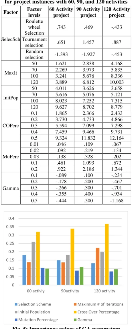
In the present study, the full profile approach was used [74]; because of considerable amount of choices, some sort of fractural factorial design was used to create suitable fraction of all possible combinations of the factor levels (orthogonal array). Orthogonal array was designed to capture the main effects for each factor level. The output of data analysis is a utility score (called part-worth) for each factor level, and part-worth provides a quantitative measure of the preference for each factor level, with larger part-worth values corresponding to greater preference. Regardless of different types of CA, maximum number of combinations (parameterization schemes) should be no more than 30 [48]. By creating orthogonal array, 25 different combinations of factor levels (cards) were created to calculate part-worths. [48] recommended the minimum number of 50 respondents for CA, so each parameterization scheme was run for 50 times. The part-worth values for sample projects are illustrated in Table 4; for example, the utility of a parameterization scheme of 60 activity project using GA with the values “roulette wheel selection’, 120, 70, 0.3, 0.02, and 0.3 for Selection Scheme, Maximum Iteration, Initial Population, Cross-Over Percentage, Mutation

Percentage, and Gamma is 0.745+3.889+5.616+5.594+0.092-0266=15.67. All the

calculations have no reversals, which means no combination (parameterization scheme) has different pattern from the main pattern calculated using CA. Based on these results, the importance of utility (part-worth) values of GA parameters for project instances with 60, 90, and 120 activities were calculated (Figure 5). For 30 activity projects, no difference was observed between the results of different parameterization schemes, so they were omitted from the chart. According to this chart, cross-over percentage is the most important attribute in all projects; the second most important attribute is the initial population for 60 and 90 activity projects and the maximum number of iterations for 120 activity projects.

Table 4:Utility (part-worth) values of GA parameters for project instances with 60, 90, and 120 activities

Factor Factor

levels

60 Activity project

SelecSch

Roulette wheel Selection

.743 .469 -.433

Tournament

selection .651 1.457 .887 Random

selection -1.393 -1.927 -.453

MaxIt

50 1.621 2.838 4.168

70 2.269 3.973 5.835

100 3.241 5.676 8.336

120 3.889 6.812 10.003

InitPop

50 4.011 3.626 3.658

70 5.616 5.076 5.121

100 8.023 7.252 7.315

120 9.627 8.702 8.779

COPerc

0.1 1.865 2.366 2.433

0.2 3.730 4.733 4.866

0.3 5.594 7.099 7.298

0.4 7.459 9.466 9.731

0.5 9.324 11.832 12.164

MuPerc

0.01 .046 .109 .067

0.02 .092 .219 .134

0.03 .138 .328 .202

0.1 .461 1.093 .672

0.2 .922 2.186 1.344

Gamma

0.1 -.089 .100 -.234

0.2 -.178 .200 -.467

0.3 -.266 .300 -.701

0.4 -.355 .400 -.934

0.5 -.444 .500 -1.168

Fig. 5:Importance values of GA parameters calculated using CA

In the first phase, by calculating the part-worth values for selected projects, the initial case base of CA-CBR optimization module was formed. At this point, three main objectives arose: first, understanding how the proposed CA-CBR module can evolve in its lifetime;

0 0.05 0.1 0.15 0.2 0.25 0.3 0.35 0.4

60 activiy 90activity 120 activity

Selection Scheme Maximum # of Iterations

Initial Population Cross Over Percentage

(10)

79

second, understanding if CBR usage is worth or not, and third, analyzing the comparison between the results before and after the integration of CA-CBR optimization module. In the second phase, the CBR cycle determines the proper parameterization scheme for new projects. There are two main criteria used to assess the performance of Hybrid CA-CBR parameterization module: evolution and effectiveness. After forming the initial case base, CBR was used to propose parameterization schemes for new projects. In order to assess the performance of CA-CBR module, two other optimization scenarios were used as baseline: Tabu search (TS) and GA with random parameterization scheme; duration of every new project was calculated 30 times using the mentioned optimization scenarios.

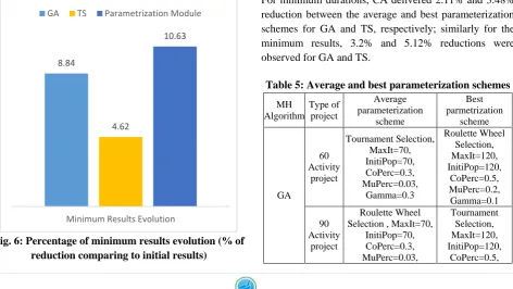
Both average and minimum calculated duration were investigated to assess the evolution and effectiveness. In order to compare the results of different projects, the reduction time (calculated duration/sum of the activity durations) was used. Figure 9 and Figure 10 show the evolution of average and minimum durations, respectively. In these figures, the evolution of both average and minimum durations is calculated for GA with random parameterization scheme; Tabu Search (TS) algorithm and parameterization scheme are suggested by CA-CBR parameterization module. In many scientific articles in the field of meta-heuristics implementation, TS is used as a benchmark algorithm to assess the performance of new optimization models. CA-CBR parameterization module shows an average 10.63% reduction for minimum results which outperform both TS and GA with average values of 4.62% and 8.84%, respectively.

Fig. 6:Percentage of minimum results evolution (% of reduction comparing to initial results)

Fig. 7:Percentage of average results evolution (% of reduction comparing to initial results)

In the third phase, to assess the effectiveness of CA

separately, the duration of sample projects (the initial case base) was calculated using GA with random parameterization scheme and TS with random parameter values for 50 times alongside with GA with optimal parameterization scheme suggested by CA. Table 5 shows the average and best parameterization schemes for sample projects with 60, 90, and 120 activities. Like the whole

CA-CBR optimization module, both reduction

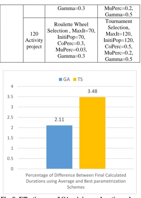
percentages related to average and minimum durations values were evaluated. Figure 8 shows the difference between minimum calculated durations using average and best parameterization schemes for both GA and TS, and Figure 9 shows similar differences for average durations. For minimum durations, CA delivered 2.11% and 3.48% reduction between the average and best parameterization schemes for GA and TS, respectively; similarly for the minimum results, 3.2% and 5.12% reductions were observed for GA and TS.

Table 5:Average and best parameterization schemes

MH Algorithm

Type of project

Average parameterization

scheme

Best parmetrization

scheme

GA

60 Activity

project

Tournament Selection, MaxIt=70, InitiPop=70, CoPerc=0.3, MuPerc=0.03,

Gamma=0.3

Roulette Wheel Selection, MaxIt=120, InitiPop=120,

CoPerc=0.5, MuPerc=0.2, Gamma=0.1

90 Activity

project

Roulette Wheel Selection , MaxIt=70,

InitiPop=70, CoPerc=0.3, MuPerc=0.03,

Tournament Selection, MaxIt=120, InitiPop=120,

CoPerc=0.5, 8.84

4.62

10.63

Minimum Results Evolution GA TS Parametrization Module

7.49

4.48

9.87

(11)

80 Gamma=0.3 MuPerc=0.2,

Gamma=0.5

120 Activity

project

Roulette Wheel Selection , MaxIt=70,

InitiPop=70, CoPerc=0.3, MuPerc=0.03,

Gamma=0.3

Tournament Selection, MaxIt=120, InitiPop=120,

CoPerc=0.5, MuPerc=0.2, Gamma=0.5

Fig. 8:Effectiveness of CA-minimum duration values

Fig. 9: Effectiveness of CA- Average Duration Values

CA has more effect on the minimum results than the average results. If the results of evolution charts (Figures 6 and 7) are combined with the results of the latter charts, some conclusions can be drawn about the effectiveness of CA in both average and minimum duration results. CBR was used in parameterization module for simulating CA, which was so time consuming (GA parameterization). Figures 8 and 9 show the total reduction percentage related to CA solely. By dividing these results to total evolution (Figures 6 and 7), CA attribution to total

evolution can be determined; accordingly, about 20% of the minimum results evolution and 30% of the average evolution can be attributed to CA, which is a considerable amount. In Figures 8 and 9, only the parameterization schemes with average CA score were compared with the best CA score parameterization schemes, and the differences between the minimum and best CA score parameterization schemes were much higher.

CONCLUSION AND RECOMMENDATIONS FOR FURTHER RESEARCHES

Defining a proper parameterization mechanism for solving RCPSP has not been a popular topic in literature. The present study used, for the first time, CA for parameterization of meta-heuristic algorithm for RCPSP. The benefit of using CA is that it enables considering the correlation between different parameterization schemes, identifying reversals, and the most important one of all: identifying the most proper parameterization scheme and assuming problem constraints and preferences including computation time, final solution score, the number of function evaluations, etc. Because of the nature of the problem, MH sessions are regarded as respondents, and full profile approach is used in CA. This study aimed to overcome the shortcomings of the main previous efforts in parameterization of MHs in scheduling problems in the area of identifying best parameterization scheme in more statistically supported way compared with randomly running MHs with different parameterization schemes. There are some recommendations for further researches: designing intelligent system that can categorize different types of RCPSP problem and propose parameterization schemes for each category; adding algorithm selection function to this model prior to proposing parameterization schemes, and developing hybrid intelligent model for parameterization that uses conjoint outcomes as learning set for other classification methods.

REFERENCES

[1] R. Klein, Scheduling of Resource-Constrained

Projects, Springer Science & Business Media, 2000.

[2] R. Słowiński, B. Soniewicki, J. Wȩglarz, DSS for

multiobjective project scheduling, Eur. J. Oper. Res. 79 (1994) 220–229.

[3] S. Rudich, A. Wigderson, Computational

Complexity Theory, American Mathematical Soc., 2004.

[4] C. Artigues, S. Demassey, E. Néron, eds.,

Resource-Constrained Project Scheduling, John Wiley & Sons, Ltd, 2008.

2.11

3.48

0 0.5 1 1.5 2 2.5 3 3.5 4

Percentage of Difference Between Final Calculated Durations using Average and Best parametrization

Schemes

GA TS

3.2

5.12

0 1 2 3 4 5 6

Percentage of Difference Between Average Durations using Average and Best Parametrization

(12)

81

[5] M. Chena, S. Yan, S.-S. Wang, Chiu-Lan, A

generalized network flow model for the multi-mode resource-constrained project scheduling problem with discounted cash flows, Eng. Optim. 47 (2015) 165–183.

[6] T. Messelis, P. De Causmaecker, An automatic

algorithm selection approach for the multi-mode resource-constrained project scheduling problem, Eur. J. Oper. Res. (2013).

[7] J. Lancaster, M. Ozbayrak, Evolutionary

algorithms applied to project scheduling problems—a survey of the state-of-the-art, Int. J. Prod. Res. 45 (2007) 425–450.

[8] R. Kolisch, S. Hartmann, Experimental

investigation of heuristics for resource-constrained project scheduling: An update, Eur. J. Oper. Res. 174 (2006) 23–37.

[9] J. Alcaraz, C. Maroto, A Robust Genetic

Algorithm for Resource Allocation in Project Scheduling, Ann. Oper. Res. 102 (2001) 83–109.

[10]Arno Sprecher, A. Drexl, Solving Multi-Mode

Resource-Constrained Project Scheduling Problems by a Simple, General and Powerful Sequencing Algorithm, Eur. J. Oper. Res. 107 (1998).

[11]R. Slowinski, Two approaches to problems of

resource allocation among project activities – A comparative study., J. Oper. Res. Soc. 31 (1980) 711–723.

[12]J. Patterson, A Comparison of Exact Approaches

for Solving the Multiple Constrained Resource, Project Scheduling Problem, Manage. Sci. 30 (1984) 854–867.

[13]A. Mingozzi, V. Maniezzo, S. Ricciardelli, L.

Bianco, An Exact Algorithm for the Resource-Constrained Project Scheduling Problem Based on a New Mathematical Formulation, (1998).

[14]R.N. Ramlogan, I.C. Goulter, Mixed Integer Model

For Resource Allocation In Project Management, Eng. Optim. 15 (1989) 97–111.

[15]K. Fleszar, K.S. Hindi, Solving the

resource-constrained project scheduling problem by a variable neighbourhood search, Eur. J. Oper. Res. 155 (2004) 402–413.

[16]Tonius Baar, P. Brucker, S. Knust, Tabu Search

Algorithms and Lower Bounds for the Resource-Constrained Project Scheduling Problem, in: S. Voß, S. Martello, I.H. Osman, C. Roucairol (Eds.), Meta-Heuristics Adv. Trends Local Search Paradig. Optim., Springer US, Boston, MA, 1998.

[17]C. Artigues, P. Michelon, S. Reusser, Insertion

techniques for static and dynamic

resource-constrained project scheduling, Eur. J. Oper. Res. 149 (2003) 249–267.

[18]M. Palpant, C. Artigues, P. Michelon, LSSPER:

Solving the Resource-Constrained Project Scheduling Problem with Large Neighbourhood Search, Ann. Oper. Res. 131 (2004) 237–257.

[19]F.F. BOCTOR, Resource-constrained project

scheduling by simulated annealing, Int. J. Prod. Res. 34 (1996) 2335–2351.

[20]K. Bouleimen, H. Lecocq, A new efficient

simulated annealing algorithm for the resource-constrained project scheduling problem and its multiple mode version, Eur. J. Oper. Res. 149 (2003) 268–281.

[21]P.R. Thomas, S. Salhi, A Tabu Search Approach

for the Resource Constrained Project Scheduling Problem, J. Heuristics. 4 (1998) 123–139.

[22]D. Debels, B. De Reyck, R. Leus, M. Vanhoucke,

A hybrid scatter search/electromagnetism meta-heuristic for project scheduling, Eur. J. Oper. Res. 169 (2006) 638–653.

[23]D. Merkle, M. Middendorf, H. Schmeck, Ant

colony optimization for resource-constrained project scheduling, IEEE Trans. Evol. Comput. 6 (2002) 333–346.

[24]Y.A. Kochetov, A.A. Stolyar, Evolutionary Local

Search with Variable Neighborhood for the Resource Constrained Project Scheduling Problem, in: 3rd Int. Work. Comput. Sci. Inf. Technol., 2003.

[25]M. Mori, C.C. Tseng, A genetic algorithm for

multi-mode resource constrained project scheduling problem, Eur. J. Oper. Res. 100 (1997) 134–141.

[26]L. Ozdamar, A genetic algorithm approach to a

general category project scheduling problem, IEEE Trans. Syst. Man Cybern. Part C (Applications Rev. 29 (1999) 44–59.

[27]S. Hartmann, Project Scheduling with Multiple

Modes: A Genetic Algorithm, Ann. Oper. Res. 102 (2001) 111–135.

[28]U. Kohlmorgen, H. Schmeck, K. Haase,

Experiences with fine‐grainedparallel genetic

algorithms, Ann. Oper. Res. 90 (1999) 203–219.

[29]A. Lova, P. Tormos, M. Cervantes, F. Barber, An

efficient hybrid genetic algorithm for scheduling projects with resource constraints and multiple execution modes, Int. J. Prod. Econ. 117 (2009) 302–316.

[30]H. Zoulfaghari, J. Nematian, N. Mahmoudi, M.

(13)

82

[31]Edmund K. Bruke, G. Kendall, eds., Search

Methodologies - Introductory Tutorials in

Optimization and Decision Support Techniques, 2014.

[32]C.M. Joo, B.S. Kim, Parallel machine scheduling

problem with ready times, due times and sequence-dependent setup times using meta-heuristic algorithms, Eng. Optim. 44 (2012) 1021–1034.

[33]X.G. Gracie, The Behavior of Simulated Annealing

in Stochastic Optimization, ProQuest, 2008.

[34]V. Yannibelli, A. Amandi, Project scheduling: A

multi-objective evolutionary algorithm that optimizes the effectiveness of human resources and the project makespan, Eng. Optim. 45 (2012) 45– 65.

[35]F. Ballestín, V. Valls, S. Quintanilla, Pre-emption

in resource-constrained project scheduling, Eur. J. Oper. Res. 189 (2008) 1136–1152.

[36]S. Hartmann, A competitive genetic algorithm for

resource-constrained project scheduling, Nav. Res. Logist. 45 (1998) 733–750.

[37]W. He, Improving user experience with case-based

reasoning systems using text mining and Web 2.0, Expert Syst. Appl. 40 (2013) 500–507.

[38]M. Kruusmaa, J. Willemson, Covering the path

space: A casebase analysis for mobile robot path planning, in: Knowledge-Based Syst., 2003: pp. 235–242.

[39]S.J. Louis, G. Li, Case injected genetic algorithms

for traveling salesman problems, Inf. Sci. (Ny). 122 (2000) 201–225.

[40]D.R. Kraay, P.T. Harker, Case-based reasoning for

repetitive combinatorial optimization problems, part I: Framework, J. Heuristics. 2 (1996) 55–85.

[41]I. Pereira, a. Madureira, Self-Optimization module

for Scheduling using Case-based Reasoning, Appl. Soft Comput. 13 (2013) 1419–1432.

[42]G. Schmidt, Case-based reasoning for production

scheduling, Int. J. Prod. Econ. 56–57 (1998) 537– 546.

[43]A. Madureira, I. Pereira, Self-Optimization for

Dynamic Scheduling in Manufacturing Systems, in: A. Madureira, I. Pereira (Eds.), Technol. Dev. Networking, Educ. Autom., Springer Netherlands, Dordrecht, 2010: pp. 421–426.

[44]E.K. Burke, B.L. MacCarthy, S. Petrovic, R. Qu,

Knowledge Discovery in a Hyper-heuristic for Course Timetabling Using Case-Based Reasoning, in: E. Burke, P. De Causmaecker (Eds.), Pract. Theory Autom. Timetabling IV, Springer Berlin Heidelberg, Berlin, Heidelberg, 2003.

[45]S. Petrovic, Y. Yang, M. Dror, Case-based

selection of initialisation heuristics for

metaheuristic examination timetabling, Expert Syst. Appl. 33 (2007) 772–785.

[46]E. Xia, I. Jurisica, J. Waterhouse, V. Sloan,

Runtime Estimation Using the Case-Based Reasoning Approach for Scheduling in a Grid Environment, in: I. Bichindaritz, S. Montani (Eds.), Case-Based Reason. Res. Dev., Springer Berlin Heidelberg, Berlin, Heidelberg, 2010.

[47]A. Schirmer, Case-based reasoning and improved

adaptive search for project scheduling, Nav. Res. Logist. 47 (2000) 201–222.

[48]J.F. Hair, W.C. Black, B.J. Babin, R.E. Anderson,

Multivariate Data Analysis (7th Edition), Prentice Hall, 2010.

[49]S. Maldonado, R. Montoya, R. Weber, Advanced

conjoint analysis using feature selection via support vector machines, Eur. J. Oper. Res. 241 (2015) 564–574.

[50]I. Endrizzi, L. Torri, M.L. Corollaro, M.L.

Demattè, E. Aprea, M. Charles, et al., A conjoint study on apple acceptability: Sensory characteristics and nutritional information, Food Qual. Prefer. 40 (2015) 39–48.

[51]J.S. Brook, J.Y. Lee, S.J. Finch, D.W. Brook,

Conjoint trajectories of depressive symptoms and delinquent behavior predicting substance use disorders., Addict. Behav. 42 (2015) 14–9.

[52]H.-P. Liew, S. Gardner, Determinants of patient

satisfaction with outpatient care in Indonesia: A conjoint analysis approach, Heal. Policy Technol. 3 (2014) 306–313.

[53]C. Atwater, R. Gopalan, R. Lancioni, J. Hunt,

Measuring supply chain risk: Predicting motor carriers’ ability to withstand disruptive environmental change using conjoint analysis, Transp. Res. Part C Emerg. Technol. 48 (2014) 360–378.

[54]E. V. Karniouchina, W.L. Moore, B. van der Rhee,

R. Verma, Issues in the use of ratings-based versus choice-based conjoint analysis in operations management research, Eur. J. Oper. Res. 197 (2009) 340–348.

[55]S. Hartmann, A self-adapting genetic algorithm for

project scheduling under resource constraints, Nav. Res. Logist. 49 (2002) 433–448.

[56]J.-L. Kim, Genetic algorithm stopping criteria for

optimization of construction resource scheduling problems, Constr. Manag. Econ. 31 (2012) 3–19.

[57]D.S. Weile, E. Michielssen, Genetic algorithm

optimization applied to electromagnetics: a review, IEEE Trans. Antennas Propag. 45 (1997) 343–353.

[58]J. Horn, N. Nafpliotis, D.E. Goldberg, A niched

(14)

83

optimization, in: Proc. First IEEE Conf. Evol. Comput. IEEE World Congr. Comput. Intell., IEEE, n.d.: pp. 82–87.

[59]I. V Karlin, A. Ferrante, H.C. Öttinger, Perfect

entropy functions of the Lattice Boltzmann method, Europhys. Lett. 47 (1999) 182–188.

[60]J.R. McDonnell, R.G. Reynolds, Evolutionary

Programming IV: Proceedings of the Fourth Annual Conference on Evolutionary Programming, MIT Press, 1995.

[61]K. Katayama, H. Sakamoto, H. Narihisa, The

efficiency of hybrid mutation genetic algorithm for the travelling salesman problem, Math. Comput. Model. 31 (2000) 197–203.

[62]M. Lang, Conjoint Analysis in Marketing

Research: Fundamentals - Methods - Applications - Critical assessment, GRIN Verlag, 2011.

[63]T. Bech-Larsen, K.G. Grunert, The perceived

healthiness of functional foods, Appetite. 40 (2003) 9–14.

[64]S. Greco, B. Matarazzo, R. Słowiński, Axiomatic characterization of a general utility function and its particular cases in terms of conjoint measurement and rough-set decision rules, Eur. J. Oper. Res. 158 (2004) 271–292.

[65]W.L. Moore, A cross-validity comparison of

rating-based and choice-based conjoint analysis models, Int. J. Res. Mark. 21 (2004) 299–312.

[66]M. Jan, T. Fu, C.L. Huang, A Conjoint/Logit

Analysis of Consumers’ Responses to Genetically Modified Tofu in Taiwan, J. Agric. Econ. 58 (2007) 330–347.

[67]S. Montani, L.C. Jain, eds., Successful Case-based

Reasoning Applications - I, Springer Berlin Heidelberg, Berlin, Heidelberg, 2010.

[68]M.M. Richter, R.O. Weber, Case-Based

Reasoning, Springer Berlin Heidelberg, 2013.

[69]S. Rudich, A. Wigderson, Computational

Complexity Theory, American Mathematical Soc., 2004.

[70]M. Kaedi, N. Ghasem-Aghaee, Biasing Bayesian

Optimization Algorithm using Case Based Reasoning, Knowledge-Based Syst. 24 (2011) 1245–1253.

[71]T.J.R. 1937- Johnson, An algorithm for the

resource constrained project scheduling problem, (1967).

[72]U. Beşikci, Ü. Bilge, G. Ulusoy, Multi-mode resource constrained multi-project scheduling and resource portfolio problem, Eur. J. Oper. Res. 240 (2015) 22–31.

[73]R. Kolisch, A. Sprecher, Project Scheduling

Problem Library(PSPLIB), (2015).

[74]J.F. Hair, W.C. Black, B.J. Babin, R.E. Anderson,