PID Controller for Vibration Reduction and
Performance Improvement of Handheld Tools
M.A.Salim, A.Noordin, A.N.Ismail, F.Munir
Abstract- This paper proposes a PID Controller to mprove handheld tools performance and at the same time reduce vibration occurs during its operation. Two experiments has been setup to record vibration of handheld drill using accelerometer placed at certain points of the hand drill. Through experiment, the obtained data was analyzed using Fast Fourier Transform (FFT) and Operational deflection shape (ODS) technique and the data being verify which gives the natural frequency at 476.07Hz which is 5.7% higher that theoretical value. From the data the PID controller is designed and tunes using Ziegler Nichols method which gives peak amplitude at 0.0144 and settling time at 0.45s. From the result it is believed that this proposed controller can reduce the vibration and give good improvement to the handheld tool performance.
Index Term-- vibration, Fast Fourier transform, PID, Ziegler Nichols.
I. INTRODUCTION
Vibration is a phenomenon that produces by a tool during operating. Study on vibration gives many spaces to learn how vibration is exactly working. Level of vibration depends on the speed of tool during operation. If higher speed is given, higher vibration will occurs. Vibration gives so many benefit and destruction. In industry, vibration is useful for their operation. For example, massaging and therapeutic application.
Usage s is very popular among the builders. For instance, hand drill is very useful in order to simplify a hard works such as in engineering fields.
When talking about hand powered portable machines, the current issues that always questioned and argued are how safe these machines to human body in term of physical and internal. A part of the issues concerning the operator safety is the transmission of vibration to the hand and arm.
In hand powered portable machines, the vibration is considered as a kinetic energy and a potential energy. It means vibration system is able to store and release energy. Hartog et.al was argued that vibration refers to mechanical
Manuscript received January 5, 2011. This research was funded by Faculty of Mechanical Engineering, Universiti Teknikal Malaysia Melaka, Malaysia.
M.A.Salim is with the Faculty of Mechanical Engineering, Universiti Teknikal Malaysia Melaka, Malaysia. (email: [email protected]).
A.Noordin is currently with Faculty of Electrical Engineering, Universiti Teknikal Malaysia Melaka, Malaysia. (email: [email protected]).
A.N.Ismail is with Faculty of Mechanical Engineering, Universiti Teknikal Malaysia Melaka, Malaysia.
F.Munir is with the Faculty of Mechanical Engineering, Universiti Teknikal Malaysia Melaka, Malaysia. (email: [email protected]).
oscillations about an equilibrium point [1], [2], [3]. The oscillations are in periodic such as the motion of a pendulum or random such as the movement of the tools.
Hand powered portable machines is an arm instrument that use hand as a support system during the operation. The feature of this instrument is it has a handle which is specially made for the convenient and safety of the users. Among the tools that are commonly used as handheld are drill, grinder, hammer, saw, axe and etc. Each tool has a handle made either on top, front or rear. For example, chainsaw has a handle on top and rear of the tool therefore it can be function well doing the cutting. Meanwhile for a drill, its handle is at the front and the rear where the rear handle is the main and the front handle act as it supporter.
Rear handle is very important for this kind of hand powered portable machines. The function of the rear handle is to control the movement of the tool. Without the rear handle, it is difficult to control the tools during operating. Vibration at the rear handle is higher compare to the other handles. This is because rear handle is commonly nearer to the motor.
II. FAST FOURIER TRANSFORM
The invention of the Fast Fourier transform (FFT) algorithm finally leads for rapid and prevalent application of experimental technique in structural dynamics. With FFT, frequency responses of a structure can be computed from the measurement of given inputs and resultant responses.
Using FFT method, the vibration can be traced. With this method, natural frequency can be found and then the spring and damping coefficient of the tool can be calculated. From FFT graph, the natural frequency is able to obtain. To find the spring and damper coefficient for this tool, equation (1) must be use to find the value of fn.
(1)
where,
n
= natural frequencyn
f
= frequencyThe value of spring coefficient would be determined from this equation,
(2) n
n f 2
m k fn
2
1
where,
k
= spring constant m = mass of toolDamping coefficient equation,
(3) (3)
where,
c = damping coefficient
= damping ratioUsing Half-Power Bandwidth equation,
(4)
(5)
Value of
f
1,f
2 andf
0can be found in FFT graph ofdamping measurement.
where,
Q
= Q factor1
f
= lower 3dB frequency (Hz)2
f
= upper 3dB frequency (Hz)0
f
= resonance frequency (Hz)III. OPERATIONAL DEFLECTION SHAPE
Operational deflection shape (ODS) is defined as the deflection of a structure at a particular frequency. However, an ODS can be defined more generally as any forced motion of two or more points on a structure. Specifying the motion of two or more points defines a shape. Stated differently, a shape is the motion of one point relative to all others. Motion is a vector quantity, which means that it has location and direction [3], [5]. This is called a Degree Of Freedom.
Measuring using ODS can give the information of:
a. The acceleration of moving machine. b. The direction of machine.
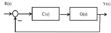
IV. PROPORTIONAL INTEGRAL DERIVATIVE CONTROLLER
Proportional Integral Derivative (PID) controller is a generic control loop feedback mechanism. This controller is widely used in industrial control system. A PID controller functions to correct the error between a measured process variable and give a corrective action that can adjust the process [2], [6]. For example, this controller can reduce the vibration on the drill.
Fig.1 PID controller plant
PID controller can be determining by using Ziegler-Nichols tuning rules:
Transfer function for PID,
(6)
where,
P
K
= Proportional gainI
K
= Integral gainD
K
= Derivative gainV. ZIEGLER-NICHOLS METHOD
Using only proportional feedback control:
i. Reduce the integrator and derivative gains to 0 (KI and KD equal to 0).
ii. Increase KP from 0 to some critical value Kp = Kcr at which sustained oscillations occur. If this does not occur, then another method has to be applied.
iii. Note the value Kcr and the corresponding period of sustained oscillation, Pcr.
TABLE I PID CONTROLLER TYPES
PID type
P
K
K
IK
DP 0.5 Kcr
0PI 0.45 Kcr
2
.
1
cr
P
0PID 0.6 Kcr
2
cr
P
8
cr
P
km
c2
1 2
0
2 1
f f
f Q
Q
) 1
1 ( )
( K s
s K K s
G D
I
P
Past research has makes a comparison for all three gains; proportional (KP), integral (KI) and derivative (KD) scheduling algorithms for a variable gain and first order time constant including time delay process. These three algorithms consist of gain scheduling (GS), fuzzy gain scheduling (FGS), and model based fuzzy gain scheduling (MFGS). GS is a gain scheduling algorithms with hard switching. FGS and MFGS are simply different ways of interpolating parameters in a gain scheduled controller. The MFGS interpolation is linear with the inverse of the controller gain, and linear with both integral and derivative time [2].
The nonlinear PID controller based on a desired response to a step set point change had been done by Zhao et.al (1993). Initially, a large control signal is desired to achieve a fast rise time, therefore the PID controller gain is large and the derivative time is small.
As the set point reach, a small controller gain is desired, therefore the overshoot is not too large. The fuzzy rules change the controller parameters based on the error and its rate of change at each time increase. [2], [3], [4].
The approach in 1992s was modified by other researchers to include dead band in between the PID controller regions where the controller parameters are linearly interpolated. Applications of these three region is designed to control a simulated pH system and show better results than a standard fixed PID controller and a rigid gain scheduler [2], [3].
Qin et.al (1995) has developed a controller logic based for PID controller for a pH process. From his simulation study, the result shows three regions designed is better than a single region designed [2].
VI. EXPERIMENT SETUP AND RESULT
A. Setup for FFT experiment
In this experiment, the accelerometers would be placed at the rear handle of the drill. Result from this experiment will give the information about vibration that occurs at the handle when the machine is running. This method can identify which area gives the highest level of vibration.
For this experiment, the material that need to be tested is BOSCH hand drill type GSB 550RE. The specification of the drill is shown below:
1. Power input = 550W 2. Impact rate = 48000 rpm 3. Weight = 1.5 kg
4. Electric motor, number of poles = 2 5. Variable speed power drill = 3000 rpm 6. Blower = 39 vanes
7. Bevel gear reduction N1 = 4/N2 = 37 8. Rolling element bearings
9. Cylindrical roller on gear box, 12 rollers/pins 10. Impact ratchet = 16 serrations
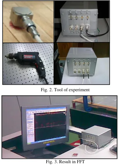
The equipments used are accelerometer, impact hammer with green tip, software, PC data acquisition system, amplifier
(4 channels), stabilize table, and rubber support. The accelerometer function is to sense or detect the vibration made by the drill. Fig. 2 and 3 shows the equipments for this experiment.
Fig. 2. Tool of experiment
Fig. 3. Result in FFT
(a) Equipment setup
(i) Put the drill on the top of the stabilize table. Use the rubber support to make sure the drill is not moving after the switch on.
(ii) Then setup the stabilize table. Open the hydraulic machine and set the rubber support at the surface of the table.
(b) Fast Fourier Transform (FFT) Analyzer Setup
(i) Firstly, setup the amplifier channel. Set channel 3 with accelerometer wire for point 1 and channel 4 with accelerometer wire for point 2.
(ii) Then attached the accelerometers at the rear handle of drill using thin layer of wax. Make sure the accelerometer is perpendicular (90 degree) to the drill surface.
(iii)Make sure all cables are connected. Turn on the constant power supplies for the accelerometer.
(c) Data acquisition
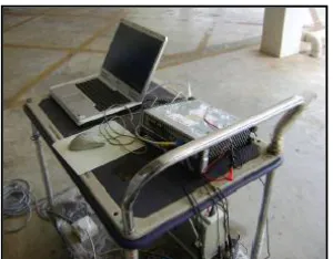
Fig. 4. DEWEsoft software
(ii) After a while, click the stop button and store the result. The result can be seen by clicking the “Analyse” button. From there, select the filename for this experiment and The Fast Fourier Transform (FFT) graph will be shown.
B. Setup for ODS experiment
Operational Deflection Shape is another method used to measure the vibration level on the rear handle of the hand drill. Six accelerometers will be placed on the handheld tool.
This experiment involved 3 important equipments:
i. 6 units of 3-axial accelerometer (KISTLER) Collect the response data in X, Y and Z direction. ii. PAK Muller-BBM FFT Analyzer
Signal from accelerometer are connected to the channel analyzer and then it would processed as required.
iii. Post-processing modal software (ME’ scope VES).
Process the data to identify the modal parameter, execute the vibration criteria, and animate the mode shapes, and Operational Deflection Shape (ODS).
Fig. 5. Experiment setup for Operational Deflection Shape (ODS)
The procedure of this experiment is:
a. All the major forcing frequencies for the synchronous forcing at x1, x2, x3 RPMs for all components such as gear mesh frequencies, bearing frequencies, ratchet impact frequencies and all components need to be calculated.
b. The analyzer must be set to a suitable maximum frequency based on the forcing frequencies.
c. Then, the accelerometer placed at the flat spot on the drill. When the drill with zero loads, the drill is run and the speed is locked at the setting. The Fast Fourier Transform spectrum where it is at least 10 averages is measured to obtain no load baseline conditions.
d. The spectrum can be stored.
e. The Fast Fourier Transform spectrum on the analyzer can be examined and all major vibration peaks and its amplitude are noted. All major frequencies include the drill x1, x2 RPMs and the gear mesh frequencies that can be identified.
VII. EXPERIMENT RESULTS AND DISCUSSION
A. Result for Fast Fourier Transform
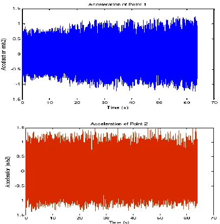
Fig. 6. Vibration at Point 1 for first measurement
Fig. 7. Vibration at point 2 for first measurement
In Figure 6 and 7, the highest vibration level occurred at frequency 476.07Hz. Point 2 produce higher vibrations than point 1. Using this value, the spring coefficient can be calculated.
B. Verification the data from Fast Fourier Transform (FFT)
Fig. 8. Theoretical data from Fast Fourier Transform (FFT)
n
Figure 8 shows the reference data (theoretical data) for this experiment. Suspected value for natural frequency is 450 Hz. Percentage of errors for this experiment has been calculated to verify the data from the experiment.
Percentage of errors is
= Experiment data – theoretical data x 100% Theoretical data
= 476.07 – 450.00 x 100% 450.00
= 5.7%
Fig. 9. Damping measurement
Resonance frequency,
f
0
8
.
62
Hz
Upper 3 dB frequency,f
2
8
.
77
Hz
Lower 3 dB frequency,f
1
8
.
46
Hz
C. Results for Operational Deflection Shape
The acceleration of the six nodal points of the rear handle of the hand drill has been successfully measured and plotted.
Fig. 10. Acceleration of the rear handle plotted in MATLAB
The acceleration of six nodal points of the rear handle of the hand drill has been measured and plotted in MATLAB. The graphs show that the highest vibration level occurred at point 2. Compare to other the graphs, point 2 produces the highest acceleration which mean the higher vibration level occurred at this point. High acceleration will gives more vibration to the drill.
VIII. APPLICATION OF PROPORTIONAL INTEGRAL
DERIVATIVE CONTROLLER
Fig. 11. Schematic diagram for the plant
Equation of motion for this system is,
(7)
The transfer function for the system is,
(8)
Use the second method of Ziegler-Nichols tuning rules,
I
K
andK
D
0
(9)The final closed loop transfer function is,
(10) From the denominator,
(11) The Routh-Hurwitz table is,
2
s
: 1.5 339940 s : 25.7K
Ps :
7 . 25 2736458KP
From the Routh-Hurwitz table, assume that the critical gain is:
(12)
The frequency of the sustained oscillation,
(13)
Hence, the period of the sustained is:
(14)
The closed-loop transfer function is given by:
(15)
Transfer function for PID controller is,
(16) where, s s s s G s s s G s s s G s K s K K s G D I P 2 0216 . 0 1667 . 4 6 . 0 ) ( 0216 . 0 144 . 0 6 . 0 6 . 0 ) ( ) 036 . 0 144 . 0 1 1 ( 6 . 0 ) ( ) 1 1 ( ) (
The closed-loop transfer function is given by: F kx x c x m F kx cu ma F f f ma ma f f F ma F s d s d . .. 3 2 25.7 339.94 10
5 . 1 1 ) ( s s s H P P K s s K s R s C 339940 7 . 25 5 . 1 ) ( ) ( 2 P K s
s 25.7 339940 5 . 1 2 1 cr K 8188 . 21 / 07 . 476 2
rad s
2 cr P ) ( ) ( 1 ) ( ) ( ) ( s H s G s G s R s C cr D cr I cr P P K P K K K 125 . 0 5 . 0 6 . 0 ) 1 1 ( )
( K s
s K K s G D I
P
1667 . 4 6 . 339940 2 7216 . 25 3 5 . 1 1667 . 4 6 . 0 2 0216 . 0 ) ( ) ( ) 339940 2 7 . 25 3 5 . 1 1667 . 4 6 . 0 2 0216 . 0 339940 2 7 . 25 3 5 . 1 ( ) 1667 . 4 6 . 0 2 0216 . 0 ( ) ( ) ( ) 339940 2 7 . 25 3 5 . 1 1667 . 4 6 . 0 2 0216 . 0 ( 1 ) 1667 . 4 6 . 0 2 0216 . 0 ( ) ( ) ( ) 339940 7 . 25 2 5 . 1 1 )( 1667 . 4 6 . 0 2 0216 . 0 ( 1 ) 1667 . 4 6 . 0 2 0216 . 0 ( ) ( ) ( ) ( ) ( 1 ) ( ) ( ) ( s s s s s s R s C s s s s s s s s s s s s R s C s s s s s s s s s R s C s s s s s s s s s R s C s H s G s G s R s C
IX. NUMERICAL ANALYSIS
This section discusses the analysis of the PID controller with the stability diagram. For the stability diagram, it used the:
i. Step Response Diagram ii. Bode Diagram
iii. Root Locus Diagram iv. Nyquist Diagram
v. Impulse Diagram
Figure 12 show the overshoot of the system is less than 10 % where this condition is obeying the regulation of the necessary of this research. That means using this result, the first objective of this research has been achieved. Besides that, the rise time of this system is 1.54 sec, peak amplitude is 1.01, overshoot is 0 %, time is 5e005 and the final value is 1.
Fig. 12. Step Response diagram for PID controller TABLE II
Result for Step Response diagram
Type Value
Rise time 1.82e005 sec Peak amplitude 1.01
Overshoot 0%
Time 5e005 sec
Settling time 3.23e005 sec
Final value 1
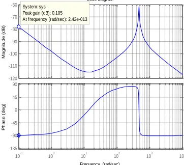
In Figure 13, the result describes the natural frequency of the system. The frequency of the system is 2.42e-013 rad/sec where this frequency refers to the natural frequency. The peak gain of this system is 75.6 dB.
Figure 14 shows two section of Root Locus diagram. In the diagram, the firstly is point 1 where the gain is 471 and the pole is -12+476i. At the second point, the gain is 462 and the pole is -11.9+476i.
Fig. 13. Bode Diagram for PID controller
Step Response Time (sec) A m p lit u d e
0 0.5 1 1.5 2 2.5 3 3.5 4 4.5 5 x 10⁵ 0 0.1 0.2 0.3 0.4 0.5 0.6 0.7 0.8 0.9 1 System: sys Peak amplitude >= 1.01 Overshoot (%): 0 At time (sec) > 5e+005 System: sys
Settling Time (sec): 3.23e+005
System: sys Rise Time (sec): 1.82e+005
10-1 100 101 102 103 104 -135 -90 -45 0 45 90 P h a s e ( d e g ) Bode Diagram
Frequency (rad/sec) -120 -110 -100 -90 -80 -70 -60 System: sys
Peak gain (dB): 0.105 At frequency (rad/sec): 2.42e-013
TABLE III Result for Bode Diagram
Fig. 14. Root Locus diagram for PID controller TABLE IV
Result for Root Locus diagram
In Figure 15, phase margin in this diagram is at -180 deg. The delay margin at this point is infinity and the frequency is 0 rad/sec.
Fig. 15. Nyquist diagram for PID controller TABLE V
Result for Nyquist diagram
Type Value
Phase margin (deg) -180 Delay margin (sec) Infinity
Frequency 0 rad/sec Closed loop stable Yes
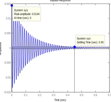
In Figure 16, peak amplitude of the system is 0.0144 at time 0 sec. The settling time for the plant is 0.45 sec.
Fig. 16. Impulse Diagram for PID controller TABLE VI
Result for Impulse Diagram
Type Value
Peak amplitude
0.0144
Time (sec) 0 Settling time
(sec)
0.45 -1000 -800 -600 -400 -200 0 200
-600 -400 -200 0 200 400 600
0.5 0.64 0.76 0.86
0.94
0.985
0.16 0.34 0.5 0.64 0.76 0.86
0.94 0.985
200 400 600 800 1e+003
System: sys Gain: 462 Pole: -11.9 - 476i Damping: 0.025 Overshoot (%): 92.5 Frequency (rad/sec): 476 System: sys Gain: 471 Pole: -12 + 476i Damping: 0.0251 Overshoot (%): 92.4 Frequency (rad/sec): 476
0.16 0.34 Root Locus
Real Axis
Im
a
g
in
a
ry
A
x
is
Nyquist Diagram
Real Axis
Im
a
g
in
a
ry
A
x
is
-1 -0.8 -0.6 -0.4 -0.2 0 0.2 0.4 0.6 0.8 1 -0.5
-0.4 -0.3 -0.2 -0.1 0 0.1 0.2 0.3 0.4 0.5
System: sys Phase Margin (deg): -180 Delay Margin (sec): Inf At frequency (rad/sec): 0 Closed Loop Stable? Yes 0 dB
-20 dB -10 dB
-6 dB -4 dB
-2 dB
20 dB 10 dB
6 dB4 dB 2 dB
Impulse Response
Time (sec)
A
m
p
lit
u
d
e
0 0.1 0.2 0.3 0.4 0.5 0.6 0.7 -0.015
-0.01 -0.005 0 0.005 0.01 0.015
System: sys Peak amplitude: 0.0144 At time (sec): 0
System: sys Settling Time (sec): 0.45
Type Value
Peak gain 0.105dB
Frequency 2.42e-013 rad/sec
Point 1 Point 2
Gain 471 Gain 462
Pole -12+476i Pole -11.9+476i Damping 0.0251 Damping 0.025 Overshoot 92.4% Overshoot 92.5% Frequency 476
rad/sec
Frequency 476 rad/sec
Point 1
X. RECOMMANDATION
For the further work of this study, comparisons with the implementation of this PID controller to the same system are necessary to look into a different condition of analysis with simulation analysis and experimental analysis. In this comparison, it can give a more accurate analysis within using software and hardware where it can handle the system to dampen the vibration. Finally, the study using software and hardware is needs to look the performance on how the improvement using PID controller into that system.
XI. CONCLUSION
Application of controller into the plant reduces the level of vibration on the handheld tools. Several types of controller were tested in order to stabilize the plant. All controllers were test one by one and lastly, the comparison for each controller will be discussed. PID controller was chosen among those controllers depend on its performance in the system of handheld tool.
The Ziegler Nichols is very useful tuning rules where this method can tune the PID controller for give a stable performance when apply this controller to the plant using the simulation in MATLAB Software. Finally the objective of this research be achieved where to reduce the vibration and at the same time give a good performance to handheld tool.
REFERENCES
[1] Hartog, Den, “Mechanical Vibrations”, Dover Publications, ISBN 0-486-647854, 1985
[2] M.A.Salim, “Design a control system to dampen the vibration in a building like structure”. Universiti Teknikal Malaysia Melaka: B.Eng Thesis, 2006.
[3] M.F Hassan, M.H Zohari, M.A Salim and C.K.E Nizwan. 2009. Identification of Vibration Level on Rear Handle of the Handheld Tool Using Operational Deflection Shape (ODS). Proceeding of ICORAFSS 2009. 90-94, 2009.
[4] Wen Tan, “Robust Controller Design and PID Tuning for Multivariable Process”, North China Power Electric University, 1996.
[5] Brian J. Schwarz & Mark H. Richardson, “Introduction to Operating Deflection Shapes”, 1999.