Nonlinear PID Triple Hyperbolic Controller Design for XY Table Ball-screw Drive System

(1)



Abstract— This paper presents an enhancement of a nonlinear PID (NPID) controller for the purpose of improving the tracking performance of an XY Table Ball-screw drive system. The new proposed control strategy which is known as NPID triple hyperbolic controller is introduced in this study. The hyperbolic algorithm of the nonlinear proportional is designed by constructing a smaller nonlinear gain when the error is small and vice versa. Meanwhile, two reciprocal hyperbolic algorithms are utilized for a nonlinear integral and nonlinear derivative. The key attribute is it will produce a smaller nonlinear gain when a higher error is released. In order to demonstrate the stability of this proposed controller, Popov stability criterion is utilized. The effectiveness of the proposed controller is verified based on the maximum tracking error and root mean square error (RMSE). The results of the proposed controller show a better tracking accuracy with an improvement of 50.58% and 36.97% compared to the NPID controller and PID controller respectively. The recommendation for future work is in term of the implementation of the optimization technique to further improve the transient aspect of this work.

Index Term— Conventional PID, maximum tracking error,

NPID, proposed NPID triple hyperbolic, RMSE

The authors would like to acknowledge the financial support by Universiti Teknikal Malaysia Melaka (UTeM) under FRGS grant with reference number

FRGS/1/2016/TK03/FKP-AMC/F00320. S.C.K.Junoh

Faculty of Manufacturing Engineering, Universiti Teknikal Malaysia Melaka, Hang Tuah Jaya, 76100 Durian Tunggal, Melaka, Malaysia,

[email protected] S.N.S.Salim

Faculty of Engineering Technology, Universiti Teknikal Malaysia Melaka, Hang Tuah Jaya, 76100 Durian Tunggal Melaka, Malaysia,

[email protected] L.Abdullah

[email protected] N.A.Anang

[email protected] T.H.Chiew

[email protected] Z.Retas

Department of Electrical Engineering, Politeknik Merlimau, KB 1031 Pej. Pos Merlimau, 77300 Melaka, Malaysia, [email protected]

1.0 INTRODUCTION

CNCmilling machines are widely used in various industrial applications, especially in the manufacturing process environment, such as drilling and cutting processes in order to produce the desired products. The basic element of a CNC machine is an XY table. This table is mostly driven indirectly by various types of motors, slightly similar to the previous study by [1]–[5]. Due to the high nonlinearities of this machine which are caused by some factors such as friction force, mechanical structure, work piece mass and cutting force [6], many types of controllers were designed. Basically, a conventional PID (proportional-integral-derivative) controller has the capacity to produce a smaller settling time, an overshoot and a steady-state error. The PID controller has been used in many applications due to its good performance and easy usage and understanding. However, the PID alone is not sufficient to make the system robust. Thus, some advance PID controllers were designed by previous researchers such as [7]–[11] with a combination of another component specifically the self-tuning adaptive controller. For example, in [10], a self-tuning adaptive PID controller was designed using a Lyapunov approach, producing a better tracking performance compared to the PID controller. On the other hand, a nonlinear design that was built in cascade with a PID known as a nonlinear PID (NPID) controller had a victorious result in terms of tracking accuracy. In [12], some advance controllers were reviewed for a precise positioning control strategy of the machine tools. Furthermore, in [13], the NPID controller was designed with a friction model in order to compensate the friction force for the XY Table Ball-screw drive system. The results showed that the Generalized Maxwell-slip (GMS) model with an NPID controller has a better performance with a smaller tracking error. In another study, the NPID controller was also presented by [14] where the nonlinear component was designed with a square root of absolute error times sign of error that enable the error sign to expand and compress. This NPID controller was tested in a simulation and experiment, resulting in a better transient response compared to the PID controller. In a subsequent study, a multi-rate nonlinear PID controller in [15] was designed using a fuzzy logic technique to enhance the NPID controller. Next, a new self-regulation nonlinear PID (SN-PID) was proposed by [16], producing an

Nonlinear PID Triple Hyperbolic Controller

Design for XY Table Ball-screw Drive System

(2)

excellent result in terms of transient response; SN-PID was improved by a factor of 2.2 times better than the NPID controller. This design’s performance was also compared to the conventional PID, NPID and sliding mode control (SMC) performances.

These evidences showed that the NPID controller is widely used recently since it produced better performance. In addition, in [17], the nonlinear function based on the exponential function combine with a PID controller showed a superior performance, even when the machine was applied with a large mass and different types of inputs, particularly the step, sinusoidal, trapezoidal and random waveforms. The nonlinear function was also introduced by [18] that presented three types of nonlinear gain namely sigmoid, hyperbolic and piecewise-linear function of the error. The previous studies proved that some nonlinear function designs with PID controllers managed to produce a better performance in nonlinear conditions. In this paper, an advancement of a nonlinear PID controller is proposed to improve the tracking accuracy of the XY table ball-screw drive system. A hyperbolic algorithm for a nonlinear proportional gain and two reciprocal hyperbolic algorithms for a nonlinear integral gain and nonlinear derivative gain are utilized in this study. These hyperbolic algorithms which use the hyperbolic secant are able to reprocess the error of the system, resulting in a changing of the nonlinear gain value that was formed by the hyperbolic formula. Thus, an NPID triple hyperbolic controller is proposed in this study. The idea of this proposed NPID triple hyperbolic controller design came from previous researcher [19], and consisted of two hyperbolic functions on a nonlinear proportional gain and nonlinear derivative gain, and an exponential function on a nonlinear integral gain. The nonlinear derivative gain that was designed in cascade with a step function was able to prevent an excessive additional damping and provide a suitable magnitude of damping when it was needed. On contrary, the nonlinear proportional gain was used to add a suitable amount of driving force, so that the system could track the input quickly. Lastly, the nonlinear integral gain was used to eliminate the steady state error that was caused by the proportional gain, others disturbances and integrator wind up.

This paper is organized as follows. In Section 2.0, the description of the XY Table Ball-screw drive system is described. In Section 3.0, the design of NPID triple hyperbolic controller is depicted in detail. In Section 4.0, the NPID triple hyperbolic controller and two other conventional controllers are tested using MATLAB/Simulink. In addition, the results are discussed in this section. Finally, in Section 5.0, this study is concluded and a recommendation is included as well.

2.0 SYSTEM MODEL

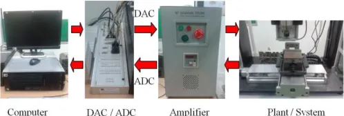
The XY Table Ball-screw drive system consists of attachment of some components such as a table, limit switches, two motors, a base, wire chains, two screws, couplers, rod tracks, and connection panels that were used in this study. The X table is 630 mm in length and 36.8 kg in mass that is installed indirectly on the screw drives horizontally. This ball-screw drive system is actuated by a servo motor that will enable it to move the table. The maximum travel distance of this X table is 300 mm. Next, an encoder with a resolution of 0.0005 mm per pulse (2000 pulse for a table movement of 1 mm) is attached to the servo motor to control the position and movement of the system. In addition, a limit switch is attached at the end of the X table for safety purpose. Furthermore, the personal computer installed with a MATLAB/Simulink and ControlDesk is linked to the dSPACE DS 1104 Digital Signal Processing (DSP) board. The DSP board or a digital analog converter (DAC/ADC) is utilized to convert the digital signal from a computer to an analog signal (servo motor) and vice versa. Then, an amplifier is linked to amplify the input signal and give the signal by a factor of ten to the actuator. The experimental setup based on the system model of an XY table ball-screw drive system is shown in Figure 1.

Fig. 1. An Experimental Setup for XY Table Ball-screw Drive System

2.1 SYSTEM IDENTIFICATION

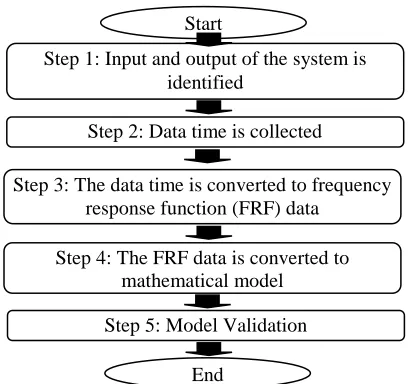
In this study, a system identification process is conducted to obtain a transfer function of the XY table ball-screw drive system. Firstly, the input and output of the system are determined based on the open-loop system. The dynamics behavior of the system based on single-input single-output (SISO) model is measured using the frequency response function (FRF). The duration for data collecting is 5 minutes. The sample frequency used is 2000 Hz, which means 2000 samples is collected in 1 second. In order to perform the system modeling, a FDIdent MATLAB toolbox is used. Thus, a second order delay is created. A flow-chart during the system identification process can be examined in Figure 2. Hence, the transfer function of the x-axis of the XY Table Ball-screw drive system is obtained as follows:

(3)

Fig. 2. A Flow-Chart of the System Identification Process

3.0 CONTROLDESIGN

The PID controller can eliminate the steady state error by increasing the integral gain [18], [20], [21], improve the transient response and reduce overshoot using the derivative gain, and improve the rise time by using proportional gain [7], [21]. However, an unpleasant response is produced when some disturbances occurred on the system. A nonlinear function is joined with the PID controller because some previous researches were required to improve the tracking accuracy of the system, for example in [22]. This function is able to tune the nonlinear gain based on system error ensuring the nonlinearities of the system can be compensated. However, one nonlinear function is not sufficient with the PID controller to further reduce the tracking error because of the limitation in the range of the allowable nonlinear gain. Thus, a controller is designed to improve the tracking accuracy of the XY Table ball-screw drive system in terms of the maximum tracking error and RMSE. For this goal, a proposed controller specifically an NPID triple hyperbolic controller is designed. This proposed controller consists of a hyperbolic function for each P, I, and D gain. Each function can generate the nonlinear gain based on the P, I, and D characteristics.

3.1 DESIGN OF NPID TRIPLE HYPERBOLIC

CONTROLLER

The NPID triple hyperbolic controller is proposed in order to improve the tracking accuracy of the system. These algorithms are designed in cascade with the P, I, D gains in order to perform a better performance based on the nonlinear characteristic of proposed controller. Thus, the triple hyperbolic controller can be expressed in (2) - (4).

KP (e) = 1 + f * (1-sech (g *eP)) (2)

KI (e) = 1. / (p + q * (1 – sech (r * eI))) (3)

KD (e) = 1. / (a + b * (1 – sech (c * eD))) (4)

These triple hyperbolic algorithms are designed for KP (e), KI (e), KD (e) in cascade with P, I, and D gain, respectively as shown in Figure 3 and is implemented in the system. This controller is analyzed in both cases, with and without disturbances. The control signal of the NPID triple hyperbolic controller can be expressed in (5) as follows:

Utriple = KP . KP(e) . e + KI . KI(e) ʃt0 e dt + KD [f(e,ė) . KD(e)] ė (5)

In addition, a step function, f(e,ė) is added in cascade with a nonlinear derivative gain which can take effect when the error has a positive value, while no effect occurs if the error has a negative value. The step function is written in (6) as follows:

function y = step_fcn (e) (6) y = 0;

if e>=0 y = 1; end

The nonlinear functions (triple hyperbolic algorithms) and step function are written in an embedded MATLAB tool on MATLAB/Simulink. The parameters of these algorithms can be determined based on the maximum nonlinear gain, k(emax) that will be described in detail in section 3.3. The algorithm in (2) stipulated that a higher nonlinear proportional gain is produced when the error is high. It enables the proportional gain to act aggressively, so that the system can respond accurately. Meanwhile, when a smaller error is released, a smaller nonlinear proportional gain will be produced, and the proportional gain will act slowly. For the algorithms in (3) and (4), the nonlinear gain acts inversely to the system error. This situation concluded that a higher nonlinear gain is needed to correct the system with a smaller error. The higher value of a nonlinear integral gain can make the output track the input that can reduce the tracking error. Furthermore, the design guideline of the NPID triple hyperbolic controller is shown in Figure 4.

Step 1: Input and output of the system is identified

Step 2: Data time is collected

Step 3: The data time is converted to frequency response function (FRF) data

Step 4: The FRF data is converted to mathematical model Step 5: Model Validation

Start

(4)

YES

Fig. 3. The NPID Triple Hyperbolic Controller Scheme

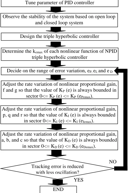
Fig. 4. Flowchart of Design Guidelines of NPID Triple Hyperbolic Controller

3.2 DETERMINATION OF HYPERBOLIC

ALGORITHMS PARAMETERS

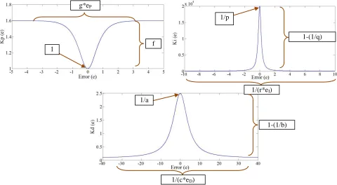
In designing the NPID triple hyperbolic controller, a determination of the hyperbolic algorithm parameters is considered. Thus, the hyperbolic algorithms parameters are obtained using a heuristic method based on a smaller maximum tracking error and less overshoot. The parameters are selected as a positive constant value and should not be zero, f and g ≠ 0, p and q and r ≠ 0, and a, b and c ≠ 0. The hyperbolic curve with a measurement parameter is shown in Figure 5. Each parameter builds a certain hyperbolic length, width and height. The hyperbolic graph is formed based on the hyperbolic parameters tuning. A smaller width will affect the nonlinear gain more, where a large adjustment of the nonlinear gain occurred although a very small error is released. Meanwhile, a large width will affect the nonlinear gain less, where a small adjustment of the nonlinear gain occurred when a very small error is released. The nonlinear proportional parameter in this study is selected at f = 0.6, g = 1.9, and ep = 2, a nonlinear integral parameter is selected at p = 5e-5_{, q = 5e} -2_{, r = 0.2, and e}

I = 0.5, and a nonlinear derivative parameter is selected at a = 0.4, b = 11, c = 0.06, and eD = 0.5. These parameters are also determined based on the range of allowable gain using Popov stability criterion that will be explained in the next section. Furthermore, the hyperbolic algorithm for KI (e) should be designed reciprocally in order to compensate the error tracking performance at a higher frequency. For a nonlinear derivative gain, the hyperbolic can be designed either reciprocally or not because this hyperbolic design has almost the same performance.

Tune parameter of PID controller

Observe the stability of the system based on open loop and closed loop system

Design the triple hyperbolic controller

Determine the kemax of each nonlinear function of NPID triple hyperbolic controller

Adjust the rate variation of nonlinear proportional gain, f and g so that the value of KP (e) is always bounded in

sector 0<= KP (e) <= KP (ePemax).

Decide on the range of error variation, eP, eI, and e D

Adjust the rate variation of nonlinear proportional gain, p, q and r so that the value of KI (e) is always bounded

in sector 0<= KI (e) <= KI (eIemax).

Adjust the rate variation of nonlinear proportional gain, a, b, and c so that the value of KD (e) is always bounded

in sector 0<= KD (e) <= KD (eDemax).

Tracking error is reduced with less oscillation?

END

(5)

Fig. 5. A Range of Hyperbolic Algorithms Curves

These hyperbolic designs were also explained in [19]. Furthermore, the nonlinear derivative gain, KD (e) is capable in reducing the oscillation in the initial part so the high nonlinear gain is selected. In Figure 6, more oscillations are produced if KD (e) is small when the parameter of ‘a’ is changed to 0.9, while less oscillation occurred when KD (e) is high, but still in the range of allowable maximum nonlinear gain. Besides, high error in the initial part is produced since small KP (e) is used when the parameter of ‘f’ is set to 0.02 and vice versa. Thus, a high nonlinear proportional gain is selected for the proportional hyperbolic algorithm.

Fig. 6. Initial Response with a High and Low Nonlinear Proportional (KP

(e)) and Nonlinear Derivative (KD (e)) Gain

3.3 STABILITY ANALYSIS FOR NPID TRIPLE HYPERBOLIC CONTROLLER

The very first step in designing this NPID triple hyperbolic controller is obtaining parameters of the PID controller. These parameters are obtained based on the gain margin, phase margin, Nyquist, sensitivity and complementary sensitivity bodes diagram that must match some requirements. The sensitivity function and complementary sensitivity function are considered to check the stability and robustness of the system [23]. Thus, the basic specification of stability range for the gain margin is 4 dB – 10 dB, the phase margin is 30° - 90°, the Nyquist plot at (-1, 0) is not encircled, the peak sensitivity is less than 6 dB and the peak complementary sensitivity is less than 2 dB. The gain of P, I, D in this case are then selected as 1.12, 0.006 and 0.007, respectively with gain margin of 8.29 dB at 209 Hz, and a phase margin of 54.4° at 80.8 Hz, the point (-1, 0) is not encircled of at the Nyquist plot, peak sensitivity of 4.91 dB at 142 Hz and peak complementary sensitivity of 0.83 dB at 107 Hz. Subsequently, the parameters of the triple hyperbolic algorithms are acquired based on the Popov stability criterion. The Popov plot is used to obtain maximum nonlinear gain so that the system is stable under conditions [13], [16]–[18], and [24]. In this study, three Popov plots are constructed to get a range of allowable gain for each nonlinear gain. The equation of Popov stability criterion can be expressed in (7) - (12).

1/a 1

g*eP

f

1/(c*eD)

1-(1/b)

1-(1/q)

(6)

The nonlinear P controller Popov plot can be expressed as follows:

ReW(jω) = k[- KP.ω2 + j.KP] / [d2.ω2 + (j – ω2)2] (7) ωImW(jω) = -k[d.KP. ω2] / [d2.ω2 + (j – ω2)2] (8)

The nonlinear I controller Popov plot can be expressed as follows:

ReW(jω) = k[d.KI] / [d2.ω2 + (j – ω2)2] (9) ωImW(jω) = -k[– KI.ω2 + j.KI] / [d2.ω2 + (j – ω2)2] (10)

The nonlinear D controller Popov plot can be expressed as follows:

ReW(jω) = k[d. KD. ω2] / [d2.ω2 + (j – ω2)2] (11) ωImW(jω) = -k[KD .ω4 – j .KD .ω2] / [d2.ω2 + (j – ω2)2] (12)

These Popov equation had been described in detail by [25]. The Popov plot for P, I and D in this case is shown in Figure 7,8, and 9 respectively with the crossing point at the zero imaginary axis obtained at (-0.616, 0) for P controller, (-1.64e-9,0) for I controller and (-0.355(-1.64e-9,0) for D controller. The Popov plot can be spotted on the right side of the tangent line of Popov plot. The real point is selected at the negative real axis. Using (13), the range of allowable nonlinear gains are obtained where 0 < KP (e) < 1.6231, 0< KI (e) < 6.0976e8 and 0 < KD (e) < 2.8098.

k (emax) = 1 / [Re.G(jω)] (13) Then, the value of KP (e), KI (e), and KD (e) are obtained as 1.5732, 3.3449e3, and 2.4695, respectively based on the range of allowable nonlinear gain and a smaller tracking error. These values are obtained after the determination of the hyperbolic algorithm parameters.

Fig. 7. Popov Plot for P Controller

Fig. 8. Popov Plot for I Controller

Fig. 9. Popov Plot for D Controller

4.0 RESULTSANDDISCUSSION

In this section, the NPID triple hyperbolic controller is tested using a MATLAB/Simulink software with a sinusoidal input to evaluate the performance of the proposed control strategy. The existing techniques such as the conventional PID and NPID controller are also tested as comparison. The tracking performances of these three controllers are analyzed and evaluated based on the maximum tracking error and root mean square error (RMSE). Three amplitudes in unit of millimeters (mm) at 5 mm, 10 mm and 15 mm and three frequencies in unit of hertz (Hz) at 0.2 Hz, 0.4 Hz and 0.6 Hz are used to verify the effectiveness of the NPID triple hyperbolic controller. In addition, three different cutting force disturbances in unit of revolution per minute (rpm) at 1500 rpm, 2500 rpm and 3500 rpm are injected to the control system with a gain of 10 in terms of robustness.

(7)

frequency. Thus, the controller gives a better performance at a low frequency.

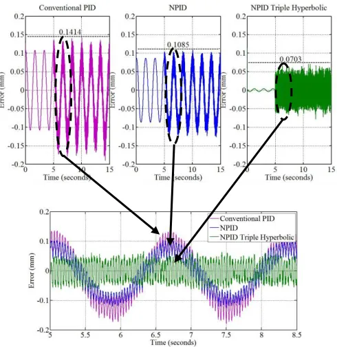
Furthermore, the result of the cutting forces is about 1500 rpm at 0.6 Hz which can be seen in Figure 11. The NPID triple hyperbolic produces the smallest maximum tracking error, 0.0703 mm, while the NPID and conventional PID produce 0.1085 mm and 0.1414 mm, respectively. The detailed results with three different spindle speeds at 1500 rpm, 2500 rpm and 3500 rpm can be viewed in Table 2. These disturbances are injected to the control system. In the case with the disturbance, the amplitude is set to 15 mm. For a 0.2 Hz of frequency, the NPID triple hyperbolic controller produces a higher maximum tracking error compared to the conventional PID and NPID at 2500 rpm and 3500 rpm, accordingly, while at 1500 rpm, the NPID triple hyperbolic controller produces a higher maximum tracking error compared to the NPID controller. However, the NPID triple hyperbolic controller achieved better tracking performance at a higher frequency (0.4 Hz and 0.6 Hz). It shows that the NPID triple hyperbolic controller has the ability to respond at a high speed. Furthermore, the results with 3500 rpm and 0.6 Hz of the proposed controller show a better tracking accuracy with the improvement of about 50.58% and 36.97% compared to the PID controller and NPID controller, respectively.

Besides, the results that are based on RMSE as shown in Table 3 and Table 4 disclosed that the NPID triple hyperbolic controller performs better tracking accuracy compared to the conventional PID and NPID controller. RMSE is represented by each point of the tracking error which is calculated as an average sum of squares of the errors. In Table 3, the NPID triple hyperbolic controller produces a smaller RMSE at a high frequency (0.6 Hz) compared to the low frequency (0.2 Hz). This result revealed that the NPID triple hyperbolic controller has a potential to track the input at a higher frequency. On the other hand, in Table 4 with the cutting force disturbance, the RMSE results for NPID triple hyperbolic controller is not much different at each frequency, but still have superior performance.

Fig. 10. Maximum Tracking Error at Amplitude 15 mm and Frequency 0.6 Hz Table I

Maximum Tracking Error

Amplitude / Frequency

Maximum Tracking Error (µm) Conventional

PID NPID

NPID Triple Hyperbolic

5 mm [µm] [µm] [µm]

0.2 Hz 13.5 13.4 0.1587

0.4 Hz 24.5 24.1 0.5760

0.6 Hz 36.0 34.7 1.2708

0.2 Hz 27.0 26.4 0.3174

0.4 Hz 49.0 46.0 1.1523

0.6 Hz 72.1 63.8 2.5416

0.2 Hz 40.5 38.7 0.4762

0.4 Hz 73.5 64.9 1.7284

(8)

Fig. 11. Simulated Maximum Tracking Error with 1500 rpm at 0.6 Hz

Table II

Maximum Tracking Error with Disturbance at Amplitude 15 mm

Spindle Speed / Frequency

Maximum Tracking Error (mm)

Conventional

PID NPID

1500 rpm [mm] [mm] [mm]

0.2 Hz 0.0744 0.0668 0.0694

0.4 Hz 0.1093 0.0897 0.0686

0.6 Hz 0.1414 0.1085 0.0703

2500 rpm [mm] [mm] [mm]

0.2 Hz 0.0614 0.0561 0.0726

0.4 Hz 0.0961 0.0803 0.0714

0.6 Hz 0.1312 0.1006 0.0705

3500 rpm [mm] [mm] [mm]

0.2 Hz 0.0500 0.0476 0.0613

0.4 Hz 0.0857 0.0741 0.0606

0.6 Hz 0.1214 0.0952 0.0600

Table III RMSE Result

Amplitude / Frequency

RMSE (µm) Error Reduction (%)

Conventional

PID NPID

NPID versus Conventio

nal PID

versus Conventional

PID

NPID Triple Hyperbolic versus

NPID

5 mm [µm] [µm] [µm] % % %

0.2 Hz 9.6000 9.5000 0.2241 1.04 97.67 97.64

0.4 Hz 17.3000 17.100

0

0.5623 1.16 96.75 96.72

0.6 Hz 25.5000 24.800

0

0.0011 2.75 99.99 99.99

10 mm [µm] [µm] [µm] % % %

0.2 Hz 19.1000 18.800

0

0.4483 1.58 97.65 97.62

0.4 Hz 34.7000 33.000

0

0.0011 4.90 99.99 99.99

0.6 Hz 51.0000 46.400

0

0.0021 9.02 99.99 99.99

15 mm [µm] [µm] [µm] % % %

0.2 Hz 28.7000 27.700

0

0.6724 3.48 97.66 97.57

0.4 Hz 52.0000 47.200

0

0.0017 9.23 99.99 99.99

0.6 Hz 76.5000 64.300

0

(9)

Table IV

RMSE with Disturbance at Amplitude 15 mm

Spindle speed / Frequency

RMSE (mm) Error Reduction (%)

Conventional

PID NPID

NPID Triple Hyperbolic NPID versus Conventional PID NPID Triple Hyperbolic versus Conventional PID NPID Triple Hyperbolic versus NPID

1500 rpm [mm] [mm] [mm] % % %

0.2 Hz 0.0381 0.0349 0.0280 8.40 26.51 19.77

0.4 Hz 0.0582 0.0507 0.0281 12.89 51.72 44.58

0.6 Hz 0.0808 0.0661 0.0282 18.19 65.10 57.34

2500 rpm [mm] [mm] [mm] % % %

0.2 Hz 0.0382 0.0351 0.0321 8.12 15.97 8.55

0.4 Hz 0.0580 0.0506 0.0321 12.76 44.66 36.56

0.6 Hz 0.0809 0.0662 0.0322 18.17 60.20 51.36

3500 rpm [mm] [mm] [mm] % % %

0.2 Hz 0.0378 0.0348 0.0277 7.94 26.72 20.40

0.4 Hz 0.0577 0.0504 0.0279 12.65 51.65 44.64

0.6 Hz 0.0803 0.0658 0.0280 18.06 65.13 57.45

5.0 CONCLUSION

In this research, a proposed control strategy, namely the NPID triple hyperbolic controller is designed to control the XY Table ball-screw drive system based on the maximum tracking error and RMSE. The purpose of this design is to reinforce the performance of the NPID controller. The hyperbolic functions for a nonlinear integral and nonlinear derivative are modified reciprocally using a hyperbolic secant function. The NPID triple hyperbolic controller can generate the error and each nonlinear gain of the PID controller will take an action to produce a better performance. The results showed that the NPID triple hyperbolic controller has a superior performance with a smaller tracking error and RMSE in most cases. Furthermore, the results of the NPID triple hyperbolic controller indicate a better tracking accuracy at a higher frequency with the improvement of about 50.58% and 36.97% compared between the PID and NPID controllers, respectively. For future work, the recommendation is to improve the transient response by utilizing an optimization technique such as the bee colony algorithm optimization.

REFERENCES

[1] X. Li, H. Zhao, X. Zhao, and H. Ding, “Dual sliding mode contouring control with high accuracy contour error estimation for five-axis CNC machine tools,” Int. J. Mach. Tools Manuf., vol. 108, pp. 74–82, 2016.

[2] C. L. Chen, M. J. Jang, and K. C. Lin, “Modeling and high-precision control of a ball-screw-driven stage,” Precis. Eng., vol. 28, no. 4, pp. 483–495, 2004.

[3] M. S. Kim and S. C. Chung, “Integrated design methodology of ball-screw driven servomechanisms with discrete controllers. Part I: Modelling and performance analysis,” Mechatronics, vol. 16, no. 8,

pp. 491–502, 2006.

[4] H. Liu, D. Lu, J. Zhang, and W. Zhao, “Receptance coupling of multi-subsystem connected via a wedge mechanism with application in the position-dependent dynamics of ballscrew drives,” J. Sound Vib., vol. 376, no. 99, pp. 166–181, 2016.

[5] G. J. Maeda and K. Sato, “Practical control method for ultra-precision positioning using a ballscrew mechanism,” Precis. Eng., vol. 32, no. 4, pp. 309–318, 2008.

[6] L. Abdullah, Z. Jamaludin, and T. Chiew, “Systematic Method for Cutting Forces Characterization for XY Milling Table Ballscrew Drive System,” Int. J., no. 6, 2012.

[7] K. M. Elbayomy, Z. Jiao, and H. Zhang, “PID controller optimization by GA and its performances on the electro-hydraulic servo control system,” Chinese J. Aeronaut., vol. 21, no. 4, pp. 378– 384, 2008.

[8] A. T. Thomas, R. P. R. Deepak, and K. S. Mohanraja, An Investigation on Modelling and Controller design of a Hydraulic press, vol. 47, no. 1. IFAC, 2014.

[9] S. N. Huang, K. K. Tan, and T. H. Lee, “A combined PID/adaptive controller for a class of nonlinear systems,” 2001.

[10] W.-D. Chang, R.-C. Hwang, and J.-G. Hsieh, “A self-tuning PID control for a class of nonlinear systems based on the Lyapunov approach,” J. Process Control, vol. 12, no. 2, pp. 233–242, 2002. [11] Z. Retas, L. Abdullah, S. Najib, S. Salim, Z. Jamaludin, and N. A.

Anang, “Tracking Error Compensation of XY Table Ball Screw Driven System Using Cascade Fuzzy P + PI,” vol. 09, no.05 September, 2016.

[12] N. A. Anang, L. Abdullah, Z. Jamaludin, Z. Retas, T. H. Chiew, S. N. S. Salim, “Precise Positioning Control Strategy of Machine Tools: A Review," unpublished

[13] T. H. Chiew, Z. Jamaludin, A. Y. Bani Hashim, N. A. Rafan, and L. Abdullah, “Friction Compensation for Precise Positioning System using Friction-Model Based Approach,” 8th MUCET 2014, no. November, pp. 10–11, 2014.

[14] M. R. Ristanovic, D. V Lazic, and I. Indin, “Nonlinear Pid Controller Modification of the Electromechanical Actuator System for Aerofin Control With a Pwm Controlled Dc Motor,” Autom.

Control Robot., vol. 7, no. Dc, pp. 131–139, 2008.

(10)

[16] S. Najib, S. Salim, M. F. Rahmat, A. A. M. Faudzi, Z. H. Ismail, and N. H. Sunar, “Position Control of Pneumatic Actuator using Self-Regulation Nonlinear PID ( SN-PID ),” vol. 2014, 2014. [17] M. F. Rahmat, “Identification and non-linear control strategy for

industrial pneumatic actuator,” Int. J. Phys. Sci., vol. 7, no. 17, pp. 2565–2579, 2012.

[18] H. Seraji, “A New Class of Nonlinear PID Controllers for Robotic Applications,” vol. 15, pp. 161–181, 1998.

[19] B. M. Isayed and M. a. Hawwa, “A nonlinear PID control scheme for hard disk drive servosystems,” 2007 Mediterr. Conf. Control

Autom., pp. 1–6, 2007.

[20] J. Patricio, O. Oliver, E. Steed, E. Quesada, A. G. Barrientos, J. Cesar, and R. Fernandez, “PID Based on Attractive Ellipsoid Method for Dynamic Uncertain and External Disturbances Rejection in Mechanical Systems,” vol. 2015, 2015.

[21] S. N. S. Salim, Z. H. Ismail, M. F. Rahmat, A. A. M. Faudzi, N. H. Sunar, and S. I. Samsudin, “Tracking performance and disturbance rejection of pneumatic actuator system,” 2013 9th Asian Control

Conf. ASCC 2013, 2013.

[22] L. Abdullah, Z. Jamaludin, J. Jamaludin, M. R. Salleh, B. Abu Bakar, M. N. Maslan, T. . Chiew, and N. a. Rafan, “Design and Analysis of Self-tuned Nonlinear PID Controller for XY Table Ballscrew Drive System,” 2nd Int. Symp. Comput. Commun.

Control Autom., vol. 3, no. 3ca, pp. 419–422, 2013.

[23] G. Karer and I. Škrjanc, “Interval-model-based global optimization framework for robust stability and performance of PID controllers,”

Appl. Soft Comput. J., vol. 40, pp. 526–543, 2016.

[24] J. Q. Liu and W. Wang, “Nonlinear Immune PID Controller and its Application to the Heat Milling System’s Material-Level Control,”

Adv. Mater. Res., vol. 383–390, pp. 743–749, 2011.

[25] Y. X. Su, D. Sun, and B. Y. Duan, “Design of an enhanced nonlinear PID controller,” Mechatronics, vol. 15, no. 8, pp. 1005– 1024, 2005.