A Genetic Algorithm Approach to Optimising Random Forests
Applied to Class Engineered Data
Eyad Elyan, Mohamed Medhat Gaber
PII:
S0020-0255(16)30578-3
DOI:
10.1016/j.ins.2016.08.007
Reference:
INS 12410
To appear in:
Information Sciences
Received date:
30 October 2015
Revised date:
25 July 2016
Accepted date:
3 August 2016
Please cite this article as: Eyad Elyan, Mohamed Medhat Gaber, A Genetic Algorithm Approach to
Optimising Random Forests Applied to Class Engineered Data,
Information Sciences
(2016), doi:
10.1016/j.ins.2016.08.007
A
C
C
E
P
T
E
D
M
A
N
U
S
C
R
IP
T
A Genetic Algorithm Approach to Optimising Random
Forests Applied to Class Engineered Data
Eyad Elyan, Mohamed Medhat Gaber
School of Computing Science and Digital Media Robert Gordon University
Riverside East, Garthdee Road, Aberdeen AB10 7GJ, UK
Email: {e.elyan,m.gaber1}@rgu.ac.uk
Abstract
In numerous applications and especially in the life science domain, examples are labelled at a higher level of granularity. For example, binary classifica-tion is dominant in many of these datasets, with the positive class denoting the existence of a particular disease in medical diagnosis applications. Such labelling does not depict the reality of having different categories of the same
disease; a fact evidenced in the continuous research in root causes and varia-tions of symptoms in a number of diseases. In a quest to enhance such diagnosis, datasests were decomposed using clustering of each class to reveal hidden cat-egories. We then apply the widely adopted ensemble classification technique Random Forests. Such class decomposition has two advantages: (1) diversifica-tion of the input that enhances the ensemble classificadiversifica-tion; and (2) improving
class separability, easing the follow-up classification process. However, to be able to apply Random Forests on such class decomposed data, three main parame-ters need to be set: number of trees forming the ensemble, number of features to split on at each node, and a vector representing the number of clusters in each class. The large search space for tuning these parameters has motivated the use of Genetic Algorithm to optimise the solution. A thorough experimental study on 22 real datasets was conducted, predominantly in a variety of life science
A
C
C
E
P
T
E
D
M
A
N
U
S
C
R
IP
T
domains. Three variations of Random Forests including the proposed method
as well as a boosting ensemble classifier were used in the experimental study. The results prove the superiority of the proposed method in boosting up the accuracy.
Keywords: Random Forests, Genetic Algorithm, Class Decomposition, Life Science
1. Introduction
Class decomposition is the process breaking down labelled datasets to a larger number of subclasses by means of applying clustering to the instances that belong to one class at a time. As such, the decomposition can be applied
to one or more classe(s) in the data set. A typical scenario is illustrated in 5
Figure 1 where a binary dataset S has been decomposed into multiple class problem (S’). Class decomposition can be traced back to 2003 when suggested to mitigate the issue of low variance classification methods [37]. However, it has been proposed in the context of biomedical data mining, as a data pre-processing phase for supervised learning. The motive is that genuine subclasses 10
can be detected, and as such the accuracy of the classification process can be enhanced. Taking two stages of development in this area of application, the work reported in [31] represents the first stage, it has bee applied to the positive class only of a number of biomedical datasets. In [18], the second stage is represented by generalising the class decomposition to all the classes in medical diagnosis 15
data sets.
In [18], Random Forests over class decomposed medical diagnosis data sets has been adopted as recent experimental studies showed its favourable results over other state-of-the-art methods [20]. In addition to the motive of finding genuine subclasses, the diversification of the data set originated from the pro-20
cess of class decomposition can further enhance the performance of ensemble classification methods, which in this case are represented by Random Forests.
A
C
C
E
P
T
E
D
M
A
N
U
S
C
R
IP
T
cluster separation is not maximised with the decomposition process. However,
class decomposition adds up a number of parameter settings that are equiva-25
lent to the number of classes. Each decomposed class can be clustered in one (the special case of not applying class decomposition to a particular class) or more subclasses. In [18], a simple setting where all classes are decomposed to the same number of clusters was used. A typical settings is shown in Figure1 where each class (A and B) in the data set S has been decomposed into two 30
subclasses (Ac1, Ac2, and Bc1, Bc2) resulting in a new decomposed data setS’.
Although this simplifies the setting, it is unlikely that this would yield the best possible results. Additionally Random Forests comes with its own parameters. Mainly the two effective settings of Random Forests is the number of trees in the ensemble, and the number of features to be assessed for goodness at each 35
split point of any tree. More details about Random Forests and its parameters
are covered in the background section of this paper.
Figure 1: Class decomposition
Realising that setting the parameters for Random Forests over class decom-posed datasets with its settings of number of clusters is an optimisation problem with a large search space,Genetic Algorithm is adopted to set all the parame-40
A
C
C
E
P
T
E
D
M
A
N
U
S
C
R
IP
T
are a relatively large number of local optima, which is the case in this problem.
The search space is exponential in the number of classes available in the data set. If the range of setting the number of subclasses is r, where r ∈ N, the number of classes in the data set is nClasses, the |mtry| is the range for the 45
number of features to use to split on at each node, and |ntree| is the range of the number of trees in the Random Forests ensemble, the search space is in
O(rnClasses|mtry||ntree|). For example, for a modest classification problem, if r= 10 (the number of subclasses attempted for each class ranges from 1 to 10),
c = 5 (the number of classes is 5), |mtry| = 10 (the range of the number of 50
features used to split on at each node),|ntree|= 100 (the range of the number of trees that form the ensemble), the search space is 105
×10×100, resulting in a large search space of 108 solutions. The contributions of this paper can be summarised as follows.
• Optimisation of Random Forests parameters applied to class decomposed 55
datasets using Genetic Algorithm. These are the number of trees and the number of features;
• optimisation of the class decomposition parameters by varying the setting of number of classes; and
• experimental validation of the proposed technique when applied to 22 60
datasets, mostly in the area of life sciences with emphasis on biomedical datasets, with exception of a number of datasets from other domains to
prove the general applicability of the method.
The paper is organised as follows. Section 2 gives the necessary background
of the computational intelligence and machine learning methods adopted in this 65
A
C
C
E
P
T
E
D
M
A
N
U
S
C
R
IP
T
2. Background
2.1. Random Forests
Ensemble classification methods have passed the test of time, and proved to be highly accurate prediction and classification techniques. According to the
winning solutions inKaggle1
, the state-of-the-art ensemble methods are Ran-75
dom Forests [11, 13] and Gradient Boosting trees [22]. Random Forests has proved superiority experimentally when compared with all widely adopted clas-sifiers including Gradient Boosting trees [20]. As an ensemble method, Random Forests adopts two methods for model diversification: (1) bootstrap sampling that applies sampling with replacement generating what is known as data repli-80
cas; and (2) each tree in the random forests chooses its node splits from a subset of the total number of features. The bootstrap sampling in the context of en-semble classification is referred to asBagging [10]. Typically Random Forests would need two parameters to set, namely, the number of trees and number of features assessed for goodness of split at each node in the tree. As a rule 85
of thumb, the number of trees is set between 100 and 500, and the number of features is set√nor log2(n) where nis the total number of features in a data set.
A number of extensions have been proposed to further enhance the perfor-mance of Random Forests [19]. In [15], the authors addressed a number of 90
Big Data problems adopting Random Forests arguing for its robustness as a classifier. Problems addressed are oversampling, undersampling, cost sensitiv-ity resulting, in class imbalancing. MapReduce was used varying a number of
settings. None of the adopted methods has shown superiority out of the exten-sive experimental study conduced in this work. In [39], the authors reported an 95
improvement in the accuracy of going-concern prediction by using a hybrid Ran-dom Forests and rough set theory approach. RanRan-dom Forests is used for feature
1Kaggle is a platform that hosts and runs machine learning competitions (https://www.
A
C
C
E
P
T
E
D
M
A
N
U
S
C
R
IP
T
selection, before the rough set method generates meaningful rules. However,
none of these methods prevailed to the point to replace the original technique, despite the slightly enhanced results reported in various papers. In a recent 100
publication it has been reported that Random Forest outperformed most of the state-of-the-art machine learning techniques in security related-application. The authors in [33] used Random Forest with weighted voting scheme along with Principle Component Analysis (PCA) to detect database access
anoma-lies, results showed that the proposed method improved false positive and false 105
negative rates and the overall accuracy of the classifier.
More recently, Random Forest gained more popularity in machine vision and visual classification tasks classification tasks [28], [32] and [25]. For example in [25] the authors proposed to decompose the multi-class classification problem into a binary classification problem in order to be solved by standard binary 110
classifiers. Evaluation on visual classification related tasks showed improvement in the accuracy.
2.2. Genetic Algorithm
Genetic Algorithm (GA) is the most widely used meta-heuristic approach for hard optimisation problems [9,38,16]. As the name suggests, GA tries to 115
emulate the genetic evolutionary process. It starts by an initial population with each individual solution is represented by a chromosome. The chromosome is decoded in most cases as a fixed-length binary string. Each chromosome
is evaluated using a fitness function designed to measure the goodness of the solution. The value of this fitness function identifies the survivors of the current 120
population, that represent the parents for the following population. Two basic operations are usually adopted as the solution strategy to generate the new population, namely, crossover and mutation.
Crossover is applied on two chromosomes at a time from the parents. Mainly
a point in the binary string is identified randomly cutting the two chromosomes, 125
A
C
C
E
P
T
E
D
M
A
N
U
S
C
R
IP
T
other one). After crossover is applied, mutation is used to generate randomness
in the solution space. It is used on one chromosome at a time flipping one of its bits. As such, the (healthy) parents generate a new population. The process is 130
then repeated for a pre-set number of populations. Numerous variants of this process have been proposed in the literature [14].
3. Related Work
Class decomposition was first proposed as a way to reduce bias in classi-fiers with high bias and low variance [37]. Noting that such classiclassi-fiers cannot 135
draw boundaries among complex class structures. Clustering is applied to ease such complexity. The technique is applied only on single classifier systems, namely, Naive Bayes, and Support Vector Machine (SVM). Clustering was ap-plied with a process that allows possible merging of the generated clusters, such
that boundaries can be easily drawn among the new classes. This allows high 140
bias classifiers to perform better. As such the quality of the clustering process in terms of cluster separation is not the ultimate goal for this research. However, more recently, in [31], the notion of class decomposition applied to biomedical datasets was proposed. The motivation in this case was that the intuition that genuine subclasses can be found in positive classes in binary biomedical datasets 145
(medical diagnosis). As such, the work in [31] used class separation as the main criteria for determining the value of the class decomposed clusters. Also it was assumed that genuine subclasses can only be found in positive classes. Those two arguments were debated in [18]. Applying class decomposition to only the positive class does not address the problem of false alarms, when a negative 150
example is classified as positive. Although finding clusters with a good
sepa-ration can enhance the classification process, it is not always desirable as the performance relies on the adopted classifier. As it is shown in [37], high bias classifiers can perform better if the decomposed clusters are re-merged. In [18], it has also been argued that class decomposition coupled with Random Forests 155
A
C
C
E
P
T
E
D
M
A
N
U
S
C
R
IP
T
cluster separation was deemed insignificant. Favourable results were reported
for applying class decomposition on medical diagnosis datasets in [18,31]. How-ever, the issue of optimal setting of class decomposition and Random Forests parameters remains an open research question. This issue is addressed in this 160
paper by adopting Genetic Algorithm.
Class decomposition was also reported in [23] by a means of a very fast neural network based method. Applying this technique, neurons adjust themselves
with each incoming observation, allowing classification of non-linearly separable classes through incremental adjustment and addition of neurons. Although the 165
method needs only one pass over the data set, it can be easily affected by noise and may lead to overfitting. The model itself can decompose classes to its components, but as noise is modelled, the number of subclasses is not optimised. Furthermore, decoupling of decomposition and classification processes as applied
in this paper allows only genuine clusters to be detected. 170
Genetic Algorithm has been used in different ways for optimising Random Forests. For example, in [8], each chromosome was a Random Forests solu-tion with a variety of trees. Applying the solusolu-tion strategy described in the background section of this paper, different solutions are generated and assessed. However, the optimisation of the number of features was not addressed. Also 175
the number of trees was not optimised directly, but a variable length chromo-some was used allowing navigation in this solution space. Favourable results were reported. Another example is reported in [6], where Genetic Algorithm was used as a feature selection phase to find the optimal set of features before applying Random Forests on the reduced feature space. The proposed method 180
was applied to a lymph disease data set. The method has proved its
applica-bility with a clear boost in accuracy over a number of other feature selection methods.
Applying machine learning in medical diagnosis has been widely reported in the literature. Recently, Azar et al [5] have thoroughly experimented a number 185
A
C
C
E
P
T
E
D
M
A
N
U
S
C
R
IP
T
vector machines (LPSVM) is superior in diagnosis aid. Results of adopting
deci-sion trees and ensemble of trees on the same data set have been reported in [4]. The study concluded that Random Forests is the most accurate method when 190
compared with single tree classifiers and ensemble of boosted trees. In this pa-per, it is argued that we can further boost the accuracy of Random Forests when an optimised setting of class decomposition is applied. As aforementioned, class decomposition can detect subclasses, resulting in better organisation of class
separability. 195
4. Methods
The two most critical parameters that define the performances of Random Forests are the number of trees (ntrees) used in each forest, and the number of features used at each split (mtry). In this paper, it is aimed to optimise
(ntrees, mtry) along with the parameterk which defines the number of clusters 200
per class in the data set. The hypothesis deriving the work reported in the paper is that by decomposing the observations within each class of a particular data set, the structure of non-linearly separable data is eased, and hence the predictive accuracy of Random Forests is boosted up.
4.1. Class Decomposition
205
Decomposing the classes of a particular data set into subclasses will be achieved
by means ofk-means clustering algorithm. Here, clustering will be used to de-compose a particular class into a set ofk-subclasses. By decomposing the class into a set of subclasses (clusters), the aim is to find the within-class similarities between different instances/observations of a data set and group them accord-210
ingly. With this approach, diversity is enhanced in the data set, and thereby the classification accuracy is improved.
A
C
C
E
P
T
E
D
M
A
N
U
S
C
R
IP
T
different ways, which may or may not share common characteristics, hence
de-composing the set of instances that are labelled as 8 into a set of clusters that share certain characteristics may certainly improve diversity and consequently improve classification accuracy. Similarly, in a medical data set with hundreds or thousands of observations, assume that each of these observations is labelled 220
to indicate whether a disease is present or not (i.e. 1 or 0 respectively). Further class decomposition could be applied and may lead to better representation of
the data (i.e. a disease is present and mild, present and severe, etc).
Formally, consider the scenario depicted in Equation1, whereX represents a set of observations, each is defined by a set of nfeatures, andY is the class 225 labels set X=
x11 x12 ..., x1n
... x22 ..., ...
... ... ... ...
xm1 ... ..., xmn
, Y = y1 .. .. ym , (1)
Now, for simplicity, lets assume that this is a binary classification that rep-resents a medical data set and thatY ∈ {1,0}, which respectively represents the presence or absence of a certain type of cancerous disease. Clearly, decom-posing the setY intoY′ will result in a larger set of classes that captures more 230
variations within classes, i.e. |Y′|>|Y|(where|Y′|,|Y|represent the number of unique class labels in the setsY′, Y respectively) and hence more diverse search
space. Some techniques reported in the literature have already shown some improvement in classification accuracy when applying class-decomposition to datasets, such as [18] and [31], however, one of the main unanswered questions 235
in this respect, is which class to decompose, and the number of subclasses in the decomposed class. For example in [31] only positive classes were considered, while in [18] all classes were decomposed using a fixed number of clusters that
was experimentally set, as previously discussed in the related work section. To answer the aforementioned questions, in this paper, the well-known stochastic 240
A
C
C
E
P
T
E
D
M
A
N
U
S
C
R
IP
T
Consider Equation1, for any machine learning algorithm, the objective is
to find a functionh(x), that maps each instance in X to its label in the setY
correctly. The ultimate aim is to maximise the accuracy ofh(x) by optimising a set of parameters. Among these parameters are thekvalues that will define 245
the new class set (Y′),
Y′= (ykvalue1 , .., y
kvalue i , ...y
kvalue m , ..., y
kvalue
L ) (2)
WhereLrepresents the number of discrete classes in the data set and ykvalue i
implies that theithclass in the setY will be decomposed intokvaluesubclasses
andkvalueis defined as in Equation3
1≤kvalue≤max, kvalue∈N (3)
Notice that kvalue here could take any value that ranges from 1 which 250
means apply no decomposition (i.e. clustering) to this class, all the way up to a
maxK as will be defined in the following sections. It is worth pointing out that with such an arrangement, for any classifier h(x) wherex belongs to classyi ,
h(x) =yijis considered as a correct classification∀j∈yisubclasses. For further
illustration, lets consider a binary classification problem (i.e. X in Equation1) 255
and suppose thatX contains 100 observation with a label setY ∈ {a, b}, and suppose that we decomposed its first class label into two subclasses, and the 2nd
class label into 3 subclasses. In addition, let’s assume that a machine learning algorithm φ is applied which resulted in a classifier hc with a 100% accuracy
represented in the form of a confusion matrix as can be seen in Equation4. 260
hc=
a1 a2 b1 b2 b3
a1 10 5 0 0 0
a2 4 31 0 0 0
b1 0 0 8 6 10
b2 0 0 9 1 16
b3 0 0 2 17 7
A
C
C
E
P
T
E
D
M
A
N
U
S
C
R
IP
T
Notice that, the confusion matrix shown in Equation 4 is often used to
compute the accuracy of a classifier by summing all elements at the diagonal and dividing it by the total number of observations (i.e. P
n i=1hii
M ). However,
the accuracy ofhc denoted byAccuracy(hc)is computed in a slightly different
way to account for the decomposition of the classes in the data set (Equation5). 265
Accuracy(h) =
PnClasses
i=0
Pki
j=0hc(i, j+ [ki−1∗i])
m (5)
Wheremis the number of observations (i.e. 100), andnClassesrepresents the number of discrete classes in the data set, whilekirepresents the number of
clusters applied to each class as will be discussed in the next section. In short, Equation5will result in summing all theboldelements of the confusion matrix in Equation4.
270
4.2. Optimised Random Forests
As discussed earlier the two most critical parameters that define the performance of Random Forests are the number of trees (ntrees) used in each forest, and the number features used at each split (mtry). Recall that the aim is to optimise
these two parameters along with the set of clusters to be applied at each class 275
label in a particular data set (i.e. thekvalue/s as formulated in Equation 2). In doing so, Genetic Algorithm is adopted to optimise these parameters.
4.2.1. Chromosome representation
For any particular data setX with a set of observations and a set of classes
Y that defines these observations (see Equation 1), and assuming thatY has
m unique classes, then a real-valued feature vector V that represents the set of parameters to be optimised in order to maximise the accuracy of Random
Forests is as shown in Equation6.
V =hyk1 1 yk
2
2 . . ym−kL1 ymkL mtry ntrees
i
(6)
whereyi∈Y andki represents thekvalue that will be set to cluster theith
A
C
C
E
P
T
E
D
M
A
N
U
S
C
R
IP
T
the optimalkvalue for each class, but also which class will be decomposed. For
example, if k was set to be equal to 1, then this simply means that no class decomposition will be applied to this particular class.
4.2.2. Solution Population
Equation6represents the solution representation that will be used to popu-285
late the GA population. In other words, an initial random set of solutions will be generated to represent different settings in order to optimise Random Forests, this population of solutions will then be evolved over a set of generations to improve and optimise the parameters and reachnear-optimal settings.
Let’s consider the Parkinson data set [27], which contains a set of obser-290
vations about people, each of them is defined by a set of attributes (23) and labelled as either healthy or having a Parkinson Disease (PD). A typical initial populations of solution may look like the one in Table2.
Table 1: Typical Solutions in a GA population
No Healthykvalue P Dkvalue nTrees MTRY
1 1 2 390 5
2 5 1 450 12
3 3 2 350 7
.. . . ... .
size . . ... .
As can be seen in Table3Healthykvaluecolumn represents thekvaluesthat the first class in the data set may take. Similarly,P Dkvaluedenotes thekvalues 295
that may be applied to the second class in the data set (PD). It is also clear that
the solution space will depend on the total number of classes that represents the data set. It is important to stress out here that a set of constraints are applied for the values that can appear within the solution representations. These include, the range of values thatkvaluecan take, which was constrained as follows: 300
A
C
C
E
P
T
E
D
M
A
N
U
S
C
R
IP
T
According to Equation7The maxkvalue has been set to equal 10, because
conducted experiments in this work in addition to previous work (i.e [18] and [31]) have shown that increasing thekvalue beyond 10 will not have significant impact on improving the results.
The number of trees has been set to range between 100 and 1000 (i.e. 100≤
305
ntrees≤1000). It was proven experimentally that the accuracy of the Random Forests do not significantly improve when increasing the number of trees beyond
500 to 1000 trees [11] therefore we set the maximum number of trees to be 1000. At the same time we set the minimum number of trees to 100.
Finally, in Equation8, the set of values that can be assigned tomtry is set as follows:
⌈0.2×n⌉ ≤mtry≤ ⌈0.8×n⌉ (8)
wherenis the total number of attributes in the data set. Notice that this range 310
will include the default settings for the Random Forests (i.e. √n, or log2(n)) all the way up to 80% of the total number of attributes.
4.2.3. Fitness Function
GA evolves the solutions iteratively and often starts with a randomly gen-erated set of solutions (population), as aforementioned. Then, this population 315
is evolved over a set of iterations, where at each of them the fitness (quality) of each solution is evaluated. The design of the fitness function is critical to the success and convergence of the GA to a good solution. In this paper, this function (Algorithm1) is designed to compute the classification accuracy of the
A
C
C
E
P
T
E
D
M
A
N
U
S
C
R
IP
T
Algorithm 1Compute the fitness of a solution
Data: Dataset, Chromosome
Result: Accuracy of the Random Forests
begin
A←−Dataset;
/* Decode the chromosome solution */
kvalues, ntrees, mtry←−decode(Chromosome);
Ac←−decomposeSet(A, kvalues); model←−f itRF(Ac, ntrees, mtry); Accuracy←−evaluate(model)
return(accuracy);
end
The fitness function outlined in Algorithm1simply decodes the chromosome solution (decode(Chromosome)) to extract the set of kvalues along with the
ntreesandmtryvalues. Following the decoding and as outlined in Algorithm1 class decomposition (decomposeSet(.., kvalues)) is applied to the data set ac-cording to the solution’s geneskvalues, then a Random Forests model will be fit 325
(f itRF(...)) on the new clustered data set and subject to the optimised number of trees of the forest and the number of features used at each split (ntreesand
mtry).
4.3. Algorithm
To wrap up this section, and before discussing our experimental setup and 330
A
C
C
E
P
T
E
D
M
A
N
U
S
C
R
IP
T
Algorithm 2Genetic Algorithm
GA(iterations, n, GA Parameters )
begin c←0 ;
i←0 ;
Generationc←generate randomnsolutions ; f itness←computeF itness(s)∀s∈Generationc;
while fitness not reached andi≤iterations do
Generationc+1←evolve(Generationc) ;
f itness←computeF itness(s)∀s∈Generationc; i←i+ 1;
end
return (fittest solution)
end
Theevolve(population) outlined in Algorithm2refers to the application of
the GA operators on the individuals (solutions) of a particular generation. This means the selection mechanism of solutions in the current generation, and the 335
application of crossover and mutation. The parameter settings of the GA will be discussed in the following section. Notice that given Algorithm2, the aim is to obtain the solution that yields the most accurate classification results (fittest solution).
5. Experiments
340
This section provides details about the different experiments that have been carried out to evaluate the proposed method. In the following sections, RF
will be used to refer to the classical Random Forests model while the proposed method will be referred to byRFGA. Secondly,RFTuned will be used to refer
to the method of tuning the RF parameters using Genetic Algorithm without 345
A
C
C
E
P
T
E
D
M
A
N
U
S
C
R
IP
T
The extensive experimental study reported in this section aims at establishing
the following:
• Class decomposition leads to a more accurate Random Forests classifier. 350
• Optimising class decomposition and Random Forests parameters is a key factor to a successful class-decomposed Random Forests.
• Affirming that class decomposition coupled with Genetic Algorithm as an optimiser is the best performing classifier among possible variations of solutions (i.e., variations of enabling or disabling decomposition, and 355
enabling or disabling parameter optimisation using Genetic Algorithm).
• The proposed method is superior when compared with state-of-the-art classifiers.
In order to establish the validity and stability of the proposed method, all
experiments discussed below have been replicated 10 times. Details of the av-360
erage classification accuracy along with standard deviation are detailed in the following sections.
5.1. Datasets
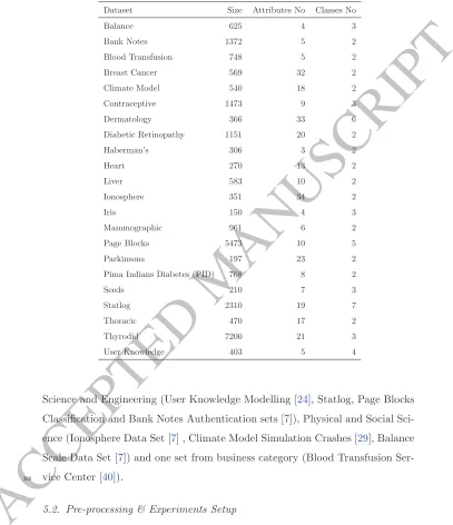
In total, 22 datasets from the UCI repository have been used in this paper [7]. As can be seen in Table2, these sets vary in terms of number of observations 365
(from 150 to 7200 instances), number of attributes (from 3 to 34 attribute) and number of class labels (from 2 to 7).
The sets shown in Table2have been selected from different domains includ-ing 14 set from the life science domain. These are mostly medical and include the
followings: Breast Cancer Wisconsin (Diagnostic) [30], Contraceptive Method 370
A
C
C
E
P
T
E
D
M
A
N
U
S
C
R
IP
T
Table 2: Details of the datasets used in the experiments
Dataset Size Attributes No Classes No
Balance 625 4 3
Bank Notes 1372 5 2
Blood Transfusion 748 5 2 Breast Cancer 569 32 2 Climate Model 540 18 2 Contraceptive 1473 9 3
Dermatology 366 33 6
Diabetic Retinopathy 1151 20 2
Haberman’s 306 3 2
Heart 270 13 2
Liver 583 10 2
Ionosphere 351 34 2
Iris 150 4 3
Mammographic 961 6 2
Page Blocks 5473 10 5
Parkinsons 197 23 2
Pima Indians Diabetes (PID) 768 8 2
Seeds 210 7 3
Statlog 2310 19 7
Thoracic 470 17 2
Thyrodid 7200 21 3
User Knowledge 403 5 4
Science and Engineering (User Knowledge Modelling [24], Statlog, Page Blocks Classification and Bank Notes Authentication sets [7]), Physical and Social Sci-ence (Ionosphere Data Set [7] , Climate Model Simulation Crashes [29], Balance Scale Data Set [7]) and one set from business category (Blood Transfusion Ser-vice Center [40]).
380
5.2. Pre-processing & Experiments Setup
The main objective of this experiment is to establish the importance of
A
C
C
E
P
T
E
D
M
A
N
U
S
C
R
IP
T
set used in this experiment was subject to pre-processing where appropriate,
in particular handling missing values in some sets using [35]and normalisation 385
where feature’s values are standardised in the range of 0 to 1 as can be seen in Equation9
zi=
xi−min(x)
max(x)−min(x) (9)
Where xi represents the ith value of feature/attribute x in the set, and
max(x), min(x) represent the maximum and minimum values in feature x, re-spectively. This step was necessary to suppress the sensitivity of k-means al-390
gorithms to outliers [18]. Once sets were pre-processed, each set has been split into two subsets, training and testing sets. The size of the training set is set to equal 80% of the original set and was divided into further two subsets (training and validation, with the validation set size set to be 20% of the original training set).
395
Figure2 depicts the workflow of the proposed methodRFGA. Notice that the training set has been used during the optimisation process (i.e. applying GA to optimise RF) while the validation set has been used to test the optimised RF during the training process. The testing set in turn has only been used to asses the resulting model (i.e. RFGA). In other words the testing set was only 400
used upon the conclusions of the training and optimisation processes, mainly to test the resulting optimised RF model.
Genetic Algorithm (GA) was implemented using [34]. GA settings used in this experiment are outlined in Table3. No other settings have been used in this paper as the optimisation of GA settings is beyond the scope of this work. 405
In order to asses the benefits of decomposing class labels on Random Forest performance, three different sets of experiments have been carried out on each set. Each of these experiments apply different methods and were replicated 10
times:
• First,RF with the default settings was applied on each set, 410
A
C
C
E
P
T
E
D
M
A
N
U
S
C
R
IP
T
Figure 2: RFGA Workflow
Table 3: GA Parameters Settings
GA Parameter Value
Population Size 500.00 Crossover 0.80
Mutation 0.10 Elitism 0.05 Max Iterations 500.00
• and finally,RF T unedwas applied which includes disabling class decompo-sition (i.e. setting thekvalueto 1) and optimising RF parameters (mtrees,
mtry) using GA.
These experimental settings are depicted in Figure3which shows the results 415
of the replicated experiments across the three different methods. Notice that for RF, the default parameters were held constant and no decomposition was applied. It is also worth noting that the ten runs in case of the RF is
repre-sented by seven red dots in Figure 3instead of ten, this is because some runs have produced the same results. . In RF GA however, the proposed method 420
A
C
C
E
P
T
E
D
M
A
N
U
S
C
R
IP
T
the y−axis of the plot) that class decomposition have been applied to both classes in this case (Breast Cancer set). In the third experimentRF T uned, the optimisation was only applied to themtryand ntreeswhilekvaluewas set to equal 1 (no decomposition).
425
The following two sections discuss and compare the results ofRF GA (the proposed method) against RF and RF T uned, where results are reported by means of average and standard deviation of the 10 replications on each set.
RFAvg, RF GAAvg and RF T unedavg denote the average runs of RF, RF GA
andRF T unedrespectively, whileXSD denotes the respective method standard
430
deviation.
The experiments will be finally concluded by comparing the performance of the RF GA against a different and rival ensemble classifier. In particular, Adaboost was used for this purposed because it proves to be one of the
state-of-the-art methods in achieving high predictive accuracy [21]. 435
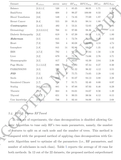
5.3. RFGA Versus RF
Comparing the predictive accuracy of both the proposed method (RF GA)
and the traditional Random Forests (RF), the results are presented in Table4. The table reports the optimal setting of the parameters that achieved the best 440
predictive accuracy for the proposed method using Genetic Algorithm. It also reports the average and standard deviation in predictive accuracy of all the 10 runs for the traditional Random Forests and the proposed method. For a fair comparison, the average predictive accuracy is used in the discussion.
It can be shown that consistent boost in the accuracy has been achieved by 445
A
C
C
E
P
T
E
D
M
A
N
U
S
C
R
IP
T
● ● ●● ●●● ● ● ●
[N,N,500,6]
[10,7,871,12] [4,2,546,10] [4,8,837,17] [5,6,565,23] [5,7,591,16] [6,4,520,12] [6,4,555,19] [7,9,724,18] [8,2,596,14] [8,4,675,18]
[1,1,344,9] [1,1,417,11] [1,1,487,13] [1,1,490,16] [1,1,522,13] [1,1,594,8] [1,1,649,9] [1,1,653,19] [1,1,746,19] [1,1643,15]
R
F
R
F
G
A
R
F
T
u
n
e
d
92 94 96 98 100
Accuracy
So
lu
ti
o
n Method
● RF
RFGA
RFTuned
Figure 3: Breast Cancer set
the pairedt-test technique. With 95% confidence, thep-value for pairedt-test is 0.003331, showing clear statistical significance. Accounting for the possibility of
the results not following the normal distribution, we also computed theWilcoxon Signed-Rank test adopting the 95% confidence. The p-value for this test is 0.001455. This also confirmed the statistical significance of the achieved results. 455
As the proposed method is composed of a number components including Genetic Algorithm and class decomposition over Random Forests, it is impor-tant to establish whether only Genetic Algorithm has the main effect, or in fact, coupling class decomposition with Genetic Algorithm is the optimal solution.
A
C
C
E
P
T
E
D
M
A
N
U
S
C
R
IP
T
Table 4: Experiments Results
Dataset Kvalues ntrees mtry RFAvg RF GAAvg RFSD RF GASD
Balance [2,3,1,1] 520 1 85.25 86.01 1.71 1.49 BankNotes [6,6] 608 2 99.27 100.00 0.33 0.00 Blood Transfusion [2,6] 549 1 74.16 77.69 1.87 1.51 Breast Cancer [6,4] 555 19 95.31 98.14 1.88 1.74
Contraceptive [2,4,5] 492 3 53.21 52.05 1.44 1.95 Dermatology [2,2,2,2,2,1] 768 11 97.66 98.36 0.74 1.13 Diabetic Retinopathy [3,2] 619 9 67.39 68.26 1.31 1.80
Haberman [3,5] 645 1 72.78 72.63 3.29 3.02 Heart [7,3] 768 4 80.08 82.83 4.18 4.74 Ionosphere [1,8] 841 14 92.86 93.73 1.35 1.42 IRIS [4,7,2] 792 1 95.19 97.04 1.56 1.56 Liver [3,2] 679 6 72.76 74.66 2.76 3.71 Mammographic [3,5] 817 2 83.07 83.39 2.04 2.36 Page Blocks [5,1,5,2,2] 696 7 97.34 97.34 0.27 0.30 PARKINSONS [3,5] 700 12 91.32 96.32 4.12 3.55
PID [7,5] 556 3 75.75 74.05 2.29 1.82 Seeds [2,4,3] 616 3 91.07 94.13 3.88 2.28 Simulated Climate [1,7] 776 7 91.71 92.40 0.00 0.97 Statlog [9,6,3,6,6,7,7] 881 9 97.88 97.93 0.48 0.29 Thoratic [[5,4] 664 6 84.61 84.67 0.56 1.49 Thyroid [3,3,3] 651 9 99.55 99.56 0.12 0.15 User knowledge [3,2,1,1] 746 3 92.44 94.00 2.21 2.68
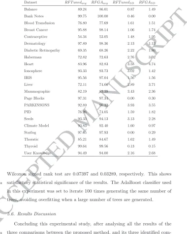
5.4. RFGA Versus RFTuned
In this set of experiments, the class decomposition is disabled allowing Ge-netic Algorithm to tune only RF’s two main parameters, namely, the number of features to split on at each node and the number of trees. This method is
compared with the proposed method of applying class decomposition with Ge-465
A
C
C
E
P
T
E
D
M
A
N
U
S
C
R
IP
T
the alternative one. Using the paired t-test with 95% confidence, the p-value
is 0.9328, and for the Wilcoxon signed rank test (also 95% confidence), thep -470
value is 0.8736, the results are not statistically significant. However, the results suggest that it is recommended to run the optimised RF without class decom-position as the first step before decomposing the classes in the data set. Then the results can be compared. This can then lead to the best possible predictive accuracy. This suggested procedure aims at distilling the cases when optimising 475
the Random Forests parameters can yield the best performance. Collectively both methods were the best performer among all the variations. As such, the practice of running both and select the best outcome has the potential of pro-ducing the strongest classifier in this family of methods. As the results show, over 3% accuracy boost can be achieved when applying class decomposition 480
(e.g., the Parkinsons set). In life science related applications, this can be an
im-portant achievement, especially those related to medical diagnosis as reported in the Parkinsons set when the optimal setting suggested a class decomposition of both the positive and the negative classes of 3 and 5 respectively.
The results reported so far assert the positive impact of class decomposition 485
on predictive accuracy of Random Forests. To establish the superiority of the proposed method over state-of-the-art ensemble methods, represented by
Ad-aBoost, the following subsection discusses this comparative experimental study.
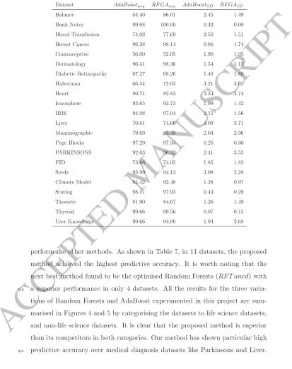
5.5. RFGA Versus AdaBoost
AdaBoost is an ensemble learning method that uses boosting of classifiers, 490
having each classifier modelled to focus on examples misclassified by previously constructed classifiers in the sequence [21]. It is among the state-of-the-art methods in achieving a high predictive accuracy. To validate the proposed method in this paper, a comparison between the two methods is conducted. Using the average of 10 runs for both methods the results are reported in Table 495
6. The results clearly suggest the superiority of the proposed method over
A
C
C
E
P
T
E
D
M
A
N
U
S
C
R
IP
T
Table 5: Tuned RF versus RFGA Performance
Dataset RF T unedavg RF GAavg RF T unedSD RF GASD
Balance 89.24 86.01 0.87 1.49 Bank Notes 99.75 100.00 0.46 0.00 Blood Transfusion 76.80 77.69 1.61 1.51 Breast Cancer 95.88 98.14 1.06 1.74 Contraceptive 54.34 52.05 1.48 1.95 Dermatology 97.89 98.36 2.13 1.13 Diabetic Retinopathy 69.35 68.26 2.22 1.80 Haberman 72.82 72.63 2.76 3.02 Heart 83.96 82.83 3.58 4.74 Ionosphere 93.33 93.73 3.02 1.42 IRIS 95.56 97.04 1.56 1.56 Liver 72.11 74.66 2.89 3.71 Mammographic 82.19 83.39 3.43 2.36 Page Blocks 97.31 97.34 0.00 0.30 PARKINSONS 92.89 96.32 3.93 3.55 PID 76.96 74.05 1.59 1.82 Seeds 93.33 94.13 3.13 2.28 Climate Model 93.83 92.40 1.60 0.97 Statlog 97.65 97.93 0.00 0.29 Thoratic 85.21 84.67 1.62 1.49 Thyroid 99.64 99.56 0.13 0.15 User Knowledge 94.49 94.00 2.16 2.68
Wilcoxon signed rank test are 0.07397 and 0.03289, respectively. This shows
satisfactory statistical significance of the results. The AdaBoost classifier used 500
in this experiment was set to iterate 100 times generating the same number of trees, avoiding overfitting when a large number of trees are generated.
5.6. Results Discussion
Concluding this experimental study, after analysing all the results of the three comparisons between the proposed method, and its three identified com-505
out-A
C
C
E
P
T
E
D
M
A
N
U
S
C
R
IP
T
Table 6: Adaboost versus RFGA Performance
Dataset AdaBoostavg RF GAavg AdaBoostSD RF GASD
Balance 84.40 86.01 2.45 1.49 Bank Notes 99.68 100.00 0.33 0.00 Blood Transfusion 74.02 77.69 2.50 1.51 Breast Cancer 96.38 98.14 0.86 1.74 Contraceptive 56.00 52.05 1.90 1.95 Dermatology 96.41 98.36 1.54 1.13 Diabetic Retinopathy 67.27 68.26 1.48 1.80 Haberman 66.54 72.63 3.21 3.02 Heart 80.71 82.83 3.34 4.74 Ionosphere 93.65 93.73 1.99 1.42 IRIS 94.98 97.04 2.15 1.56 Liver 70.81 74.66 3.09 3.71 Mammographic 79.69 83.39 2.04 2.36 Page Blocks 97.29 97.34 0.25 0.30 PARKINSONS 92.63 96.32 2.41 3.55 PID 73.66 74.05 1.85 1.82 Seeds 93.99 94.13 3.08 2.28 Climate Model 94.42 92.40 1.28 0.97 Statlog 98.11 97.93 0.43 0.29 Thoratic 81.90 84.67 1.26 1.49 Thyroid 99.66 99.56 0.07 0.15 User Knowledge 99.66 94.00 1.94 2.68
perform the other methods. As shown in Table7, in 11 datasets, the proposed
method achieved the highest predictive accuracy. It is worth noting that the next best method found to be the optimised Random Forests (RF T uned) with a superior performance in only 4 datasets. All the results for the three varia-510
tions of Random Forests and AdaBoost experimented in this project are sum-marised in Figures4and5by categorising the datasets to life science datasets, and non-life science datasets. It is clear that the proposed method is superior
A
C
C
E
P
T
E
D
M
A
N
U
S
C
R
IP
T
This can be attributed to the complexity of the problem, and that indeed these
datasets can be naturally decomposed to its subclasses, that in turn facilitates classification using Random Forests.
Table 7: Winning sets across all experiments
Dataset RF GAavg RFavg RF T unedavg AdaBoostavg
Bank Notes 100.00 99.27 99.75 99.68 Blood Transfusion 77.69 74.16 76.80 74.02 Breast Cancer 98.14 95.31 95.88 96.38 Dermatology 98.36 97.66 97.89 96.41 Ionosphere 93.73 92.86 93.33 93.65 IRIS 97.04 95.19 95.56 94.98 Liver 74.66 72.76 72.11 70.81 Mammographic 83.39 83.07 82.19 79.69 Page Blocks 97.34 97.34 97.31 97.29 PARKINSONS 96.32 91.32 92.89 92.63 Seeds 94.13 91.07 93.33 93.99
5.7. Implementation
A framework was implemented using R where several packages have been 520
utilised. These include amongst other libraries: randomForest package [26] which implements Brieman and Cutler Random Forests for Classification and Regression, and the GA package [34] which allows parallel implementation of the Genetic Algorithm. Table3 shows the parameters settings that have been
used for this experiment. AdaBoost package [1] which has been used to build 525
the AdaBoost ensemble. For handling missing values [35] and [36] were used to impute missing values.
The framework was designed to make use of the multicore facilities by util-ising R packages that enable parallel execution of the code (i.e. [2]). It is worth noting that the proposed method is scalable, as individual chromosomes 530
A
C
C
E
P
T
E
D
M
A
N
U
S
C
R
IP
T
● ● ● ● ● ● ● ● ● ● ● ● ● ● ● ● ● ● ● ● ● ● ● ● ● ● ● ●Breast Cancer Contraceptive Dermatology Diabetes PID
Diabetic Haberman Heart IRIS
Liver Mamographic Parkinsons Seeds
Thoratic Thyroid 50 60 70 80 90 100 50 60 70 80 90 100 50 60 70 80 90 100 50 60 70 80 90 100 R F R F T u n e d R F G A A d a Bo o st R F R F T u n e d R F G A A d a Bo o st Experiment A ccu ra cy
Experiment RF RFTuned RFGA AdaBoost
Figure 4: Life science Datasets Results
other trees. Consequently, only the number of iterations of the Genetic Algo-rithm is the main factor in the time needed to find the final solution. This is the case with all evolutionary optimisation methods, that are built in a sequence of 535
generations.
A
C
C
E
P
T
E
D
M
A
N
U
S
C
R
IP
T
● ● ● ● ● ● ● ● ● ● ●Balance Bank Notes Blood Trans
Climate Model Ionosphere Page Blocks
Statlog U Knowledge
70 80 90 100 70 80 90 100 70 80 90 100 R F R F T u n e d R F G A A d a Bo o st R F R F T u n e d R F G A A d a Bo o st Experiment A ccu ra cy
Experiment RF RFTuned RFGA AdaBoost
Figure 5: Non-Life science Datasets Results
out on 24 core VMWare Virtual Server with 48GB of RAM. 540
6. Conclusion and Future Work
The paper proposed a three-component system for enhancing the
A
C
C
E
P
T
E
D
M
A
N
U
S
C
R
IP
T
data set. Setting the number of clusters for each class has its own effect on the
predictive accuracy. Random Forests which is a highly accurate classification method is the second component of the proposed system. It requires two main parameters to be set: (1) number of trees in the ensemble, and (2) the number of features sampled randomly at each node split of each tree. Collectively the 550
number of parameters to set is equal to number of classes in the data set, in ad-dition to the two Random Forests parameters. Realising the large search space
generated from setting all these parameters which is exponential in the number of classes in a a data set, there is a clear need for an effective optimisation method. Thus, Genetic Algorithm is used as our third component. The system 555
was applied to 22 datasets predominantly in the area of life sciences, and the re-sults proved the effectiveness of the proposed hybrid machine learning technique in enhancing the predictive accuracy.
We can identify a number of future directions for this research as follows. Experimenting the hybrid method to other application domains in life sciences 560
such as gene expression datasets is one direction. The optimisation of GA pa-rameters is another direction which may lead to further improvements of the RF performance. Also the adoption of other population-based meta-heuristic methods can be used to compare the effectiveness of a number of optimisation
techniques . Finally, the use of other high performing machine learning algo-565
rithms like Gradient Boosting trees, or Support Vector Machines (SVM) can be explored instead of Random Forests.
References
[1] E. Alfaro, M. G´amez, N. Garc´ıa, adabag: An R package for classification
with boosting and bagging, Journal of Statistical Software 54 (2) (2013) 570
1–35.
URLhttp://www.jstatsoft.org/v54/i02/
par-A
C
C
E
P
T
E
D
M
A
N
U
S
C
R
IP
T
allel package, r package version 1.0.8 (2014).
URLhttp://CRAN.R-project.org/package=doParallel
575
[3] B. Antal, A. Hajdu, An ensemble-based system for automatic screening of
diabetic retinopathy, Knowledge-Based Systems 60 (2014) 20 – 27.
[4] A. T. Azar, S. M. El-Metwally, Decision tree classifiers for automated
med-ical diagnosis, Neural Computing and Applications 23 (7-8) (2013) 2387– 2403.
580
[5] A. T. Azar, S. A. El-Said, Performance analysis of support vector machines
classifiers in breast cancer mammography recognition, Neural Computing and Applications 24 (5) (2014) 1163–1177.
[6] A. T. Azar, H. I. Elshazly, A. E. Hassanien, A. M. Elkorany, A random forest classifier for lymph diseases, Computer methods and programs in 585
biomedicine 113 (2) (2014) 465–473.
[7] K. Bache, M. Lichman, UCI machine learning repository (2013).
URLhttp://archive.ics.uci.edu/ml
[8] M. Bader-El-Den, M. Gaber, Garf: towards self-optimised random forests, in: Neural Information Processing, Springer, 2012, pp. 506–515.
590
[9] I. Boussa¨ıD, J. Lepagnot, P. Siarry, A survey on optimization metaheuris-tics, Information Sciences 237 (2013) 82–117.
[10] L. Breiman, Bagging predictors, Machine learning 24 (2) (1996) 123–140.
[11] L. Breiman, Random forests, Mach. Learn. 45 (1) (2001) 5–32.
URLhttp://dx.doi.org/10.1023/A:1010933404324
595
[12] M. Charytanowicz, J. Niewczas, P. Kulczycki, P. A. Kowalski, S. Lukasik, S. ˙Zak, Information Technologies in Biomedicine: Volume 2, chap.
A
C
C
E
P
T
E
D
M
A
N
U
S
C
R
IP
T
[13] D. R. Cutler, T. C. Edwards Jr, K. H. Beard, A. Cutler, K. T. Hess, 600
J. Gibson, J. J. Lawler, Random forests for classification in ecology, Ecology 88 (11) (2007) 2783–2792.
[14] L. D. Davis, K. De Jong, M. D. Vose, L. D. Whitley, Evolutionary algo-rithms, vol. 111, Springer Science & Business Media, 2012.
[15] S. del Ro, V. Lpez, J. M. Bentez, F. Herrera, On the use of mapreduce for 605
imbalanced big data using random forest, Information Sciences 285 (2014) 112 – 137, processing and Mining Complex Data Streams.
[16] A. E. Eiben, J. E. Smith, Introduction to evolutionary computing, Springer Science & Business Media, 2003.
[17] M. Elter, R. Schulz-Wendtland, T. Wittenberg, The prediction of breast 610
cancer biopsy outcomes using two CAD approaches that both emphasize an intelligible decision process, Medical Physics 34 (2007) 4164.
[18] E. Elyan, M. M. Gaber, A fine-grained random forests using class decom-position: an application to medical diagnosis, Neural Computing and Ap-plications (2015) 1–10.
615
URLhttp://dx.doi.org/10.1007/s00521-015-2064-z
[19] K. Fawagreh, M. M. Gaber, E. Elyan, Random forests: from early devel-opments to recent advancements, Systems Science & Control Engineering: An Open Access Journal 2 (1) (2014) 602–609.
[20] M. Fern´andez-Delgado, E. Cernadas, S. Barro, D. Amorim, Do we need 620
hundreds of classifiers to solve real world classification problems?, Journal of Machine Learning Research 15 (2014) 3133–3181.
URLhttp://jmlr.org/papers/v15/delgado14a.html
[21] Y. Freund, R. E. Schapire, et al., Experiments with a new boosting
A
C
C
E
P
T
E
D
M
A
N
U
S
C
R
IP
T
[22] J. H. Friedman, Stochastic gradient boosting, Computational Statistics &
Data Analysis 38 (4) (2002) 367–378.
[23] S. Jaiyen, C. Lursinsap, S. Phimoltares, A very fast neural learning for
clas-sification using only new incoming datum, Neural Networks, IEEE Trans-actions on 21 (3) (2010) 381–392.
630
[24] H. T. Kahraman, S. Sagiroglu, I. Colak, The development of intuitive knowledge classifier and the modeling of domain dependent data, Know.-Based Syst. 37 (2013) 283–295.
[25] T. Li, B. Ni, X. Wu, Q. Gao, Q. Li, D. Sun, On random hyper-class random forest for visual classification, Neurocomputing 172 (2016) 281 – 635
289.
URL http://www.sciencedirect.com/science/article/pii/
S0925231215005901
[26] A. Liaw, M. Wiener, Classification and regression by randomforest, R News 2 (3) (2002) 18–22.
640
URLhttp://CRAN.R-project.org/doc/Rnews/
[27] M. A. Little, P. E. McSharry, S. J. Roberts, D. A. Costello, I. M. Moroz, Exploiting nonlinear recurrence and fractal scaling properties for voice
dis-order detection, BioMedical Engineering OnLine 6 (1) (2007) 1–19.
URLhttp://dx.doi.org/10.1186/1475-925X-6-23
645
[28] X. Liu, M. Song, D. Tao, Z. Liu, L. Zhang, C. Chen, J. Bu, Random forest
construction with robust semisupervised node splitting, IEEE Transactions on Image Processing 24 (1) (2015) 471–483.
[29] D. D. Lucas, R. Klein, J. Tannahill, D. Ivanova, S. Brandon, D. Domyan-cic, Y. Zhang, Failure analysis of parameter-induced simulation crashes in 650
climate models, Geoscientific Model Development 6 (4) (2013) 1157–1171.
A
C
C
E
P
T
E
D
M
A
N
U
S
C
R
IP
T
[30] O. L. Mangasarian, W. N. Street, W. H. Wolberg, Breast cancer
diagno-sis and prognodiagno-sis via linear programming, OPERATIONS RESEARCH 43 (1995) 570–577.
655
[31] I. Polaka, Clustering algorithm specifics in class decomposition, in: Applied Information and Communication Technology, 2013,Proceedings of the 6th International Scientific Conference, 2013, pp. 29–36.
[32] M. Ristin, M. Guillaumin, J. Gall, L. V. Gool, Incremental learning of random forests for large-scale image classification, IEEE Transactions on 660
Pattern Analysis and Machine Intelligence 38 (3) (2016) 490–503.
[33] C. A. Ronao, S.-B. Cho, Anomalous query access detection in rbac-administered databases with random forest and {PCA}, Information Sciences (2016) –.
URL http://www.sciencedirect.com/science/article/pii/
665
S0020025516304595
[34] L. Scrucca, GA: A package for genetic algorithms in R, Journal of Statistical Software 53 (4) (2013) 1–37.
URLhttp://www.jstatsoft.org/v53/i04/
[35] D. J. Stekhoven, missForest: Nonparametric Missing Value Imputation 670
using Random Forest, r package version 1.4 (2013).
[36] D. J. Stekhoven, P. Buehlmann, Missforest - non-parametric missing value imputation for mixed-type data, Bioinformatics 28 (1) (2012) 112–118.
[37] R. Vilalta, M.-K. Achari, C. F. Eick, Class decomposition via clustering: a new framework for low-variance classifiers, in: Data Mining, 2003. ICDM 675
2003. Third IEEE International Conference on, IEEE, 2003, pp. 673–676.
[38] D. Whitley, A genetic algorithm tutorial, Statistics and computing 4 (2)
A
C
C
E
P
T
E
D
M
A
N
U
S
C
R
IP
T
[39] C.-C. Yeh, D.-J. Chi, Y.-R. Lin, Going-concern prediction using hybrid
random forests and rough set approach, Information Sciences 254 (2014) 680
98 – 110.
[40] I.-C. Yeh, K.-J. Yang, T.-M. Ting, Knowledge discovery on rfm model using bernoulli sequence, Expert Syst. Appl. 36 (3) (2009) 5866–5871.
[41] M. Ziba, J. M. Tomczak, M. Lubicz, J. witek, Boosted {SVM} for ex-tracting rules from imbalanced data in application to prediction of the 685