Generating input data for microstructure modelling: A deep learning approach using generative adversarial networks

Generating input data for microstructure modelling:

A deep learning approach using generative

adversarial networks

Felix Pütz1 , Manuel Henrich1, Niklas Fehlemann1, Andreas Roth1and Sebastian Münstermann1

1 _{Integrity of Materials and Structures, RWTH Aachen University}

* Correspondence: [email protected]

Abstract: For the generation of representative volume elements a statistical description of the relevant parameters is necessary. These parameters usually describe the geometric structure of a single grain. Commonly, parameters like area, aspect ratio and slope of the grain relative to the rolling direction are applied. However, usually simple distribution functions like log normal or gamma distribution are used. Yet, these do not take the interdependencies between the microstructural parameters into account. To fully describe any metallic microstructure though, these interdependencies between the singular parameters need to be accounted for. To accomplish this representation, a machine learning approach was applied in this study. By implementing a Wasserstein generative adversarial network, the distribution, as well as the interdependencies could accurately be described. A validation scheme was applied to verify the excellent match between microstructure input data and synthetically generated output data.

Keywords:Microstructure Modelling; Representative Volume Elements; DP-steel; Machine Learning; Deep Learning; Wasserstein GAN

1. Introduction

For modern applications, the microstructures and properties of steels become exceedingly complex, utilizing multiple phases and alloying concepts to improve mechanical properties for the specific use case. Even more basic materials, like dual-phase steels show complex correlations between their microstructure and mechanical properties, as well as their damage behaviour. The morphology of a given dual-phase microstructure plays an important role in the damage mechanisms, namely initiation and accumulation [1]. Multiple parameters have been identified that each play an important role, like grain size, martensite content, or grain shape. However, it is a very complex task to separate the multiple microstructural influences experimentally. To seperately investigate each of the possible influencing factors, a numerical approach is more useful and commonly applied.The method of microstructure modelling has been of major interest in recent years and is continually developed. Commonly, two different methods are applied: Modeling the real microstructure and representing the microstructure by statistical distributions. For the first approach, the real microstructure is modeled based on a microstructural analysis. For that procedure, mostly scanning electron microscopy is used to gather the required information in a suitable resolution [2]. The second option requires a statistical analysis of the base material. The acquired statistical information is then used to create small volume elements that show a good statistical representation of the microstructure[3]. A key requirement for these volume elements is that they need to contain enough information of the microstructure, while also being small enough to be clearly differentiated from the macroscopic structural dimension [4]. Due to this requirement, it is necessary to create statistical descriptions of the microstructure to reasonably represent it. If a 2D RVE is to be created the required data can be acquired from pictures of the microstructure, either via light optical microscopy (LOM) or scanning electron microscopy (SEM).

Since the parameters of interest are on a singular grain level, SEM is used commonly. Here, multiple different detectors can be applied, while the electron backscatter diffraction (EBSD) detector delivers more in-depth information of each grain. The grain parameters that are most commonly applied in the creation of RVEs are the grain size, its shape (elongation) and the slope of the grain describing the angle between the main axis of the grain and the x-axis of the picture (or the rolling direction). For three dimensional RVE these parameters need to be determined in all three directions in space. This can be done by serial sectioning, where the sample rotates inside a strong radiation beam and is scanned slice by slice, until a projection of the material can be acquired [5]. This method is, however, a very complex and time-consuming task. Thus, pictures from all three directions in space are often taken to create statistical distribution functions of the desired parameters depending on the respective spatial direction.

For the generation of the RVE model, the statistical distribution of the microstructure needs to be translated from the material to input parameters. For that reason, the parameters are commonly described by distribution functions that follow a log-normal distribution or a gamma distribution. Most often, histograms are used to fit the distribution functions to. It has to be mentioned though, that histograms are very dependent on the bin size. Thus the resulting distribution function is also depending on the bin size. Therefore, Kernel Density Estimation (KDE) should be the prevalent method, since they deliver robust values, where every data point is weighted by a function depending on the Kernel chosen (e.g. Gaussian) [6]. Modern RVE generation algorithms take many parameters into account that describe the grain shape [7–10] . The input for these parameters are separate, independent distribution functions of the applied parameters. Most materials, however show some kind of interdependence of the parameters among each other. Thus this study analysed the interdependence of the parameters to then find a deep learning solution afterwards, that is able to describe the distribution of singular parameters as well as the interdependencies.

Figure 1.EBSD of steel DP800 where x-axis is the rolling direction (RD) and y-axis is the sheet normal (SD) [11].

2. Analysis of the input data from the real microstructure

functions of the input parameters are created and used to generate a discrete amount of input parameters for the microstructure modelling. For the present study, a dual-phase steel (DP800) was utilized as the base material, since multiple important parameters are present for the characterization of the microstructure. InFigure 1the microstructure of the DP800 steel is depicted as an EBSD picture. In this study only one direction in space was chosen for the analysis, since strong differences between different directions might apply. The rolling direction (RD) - sheet normal (SN) plane is the chosen, since it shows the elongation of the grains and therefore a more complex microstructure.

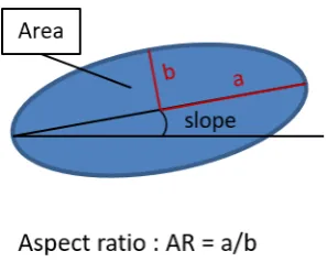
From this picture it can already be seen, that multiple different parameters are inherent to the microstructure. For any kind of microstructure modelling geometric parameters of the grains are needed as input. InFigure 2the geometric parameters of each individual grain are depicted. Probably the most important aspect is the grains specific area, since the grain size also influences mechanical properties. Apart form the size, the slope is an important factor and describes the tilt of a grain towards the x-axis of the EBSD picture taken, in this case the rolling direction (RD), where angles close to 0◦or 180◦ means an elongation of the grain along the rolling direction. The last parameter is the aspect ratio (AR), the ratio of the two half-axis a and b. A high AR stands for a bigger elongation, while an AR of 1 describes a circle. Apart from these geometrical factors, there are further material specific characteristics. The first is the grain orientation this is especially important when a texture is present in the material. Next are the different phases, in the case of DP800, ferrite and martensite. Additionally neighbourhood relations between the grains might be taken into account. All of the parameters mentioned above can be gathered from the data generated by EBSD measurement. From this measurement a list of grains and their corresponding characteristics can be obtained that is afterwards used for further analysis.

Figure 2.Schematic representation of a single grain with the associated shape parameters .

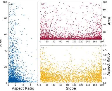
Figure 3.KDE plots of the dependencies between the three main grain parameters, grain size, aspect ration and slope.

The scatter plots show the connectivity between the main parameters. InFigure 3a) the grain size against the aspect ratio is depicted. Most grains are concentrated in the bottom left corner meaning they posses a relatively small area and aspect ratio. However, the most noticeable property is the fact, that grains above 20µm2grain size show a tendency towards smaller aspect ratios of 2.5 or lower, while for the smaller grains higher aspect ratios become increasingly likely. Another strong connection is visible inFigure 3c). Here it is identifiable, that more grains have a slope around 0◦or 180◦respectively, which both go along the x-axis (RD). Especially notable is the fact that towards a slope of 90◦, which goes perpendicular to the RD, a significantly smaller quantity of grains show aspect ratios above 2.5. This means, that grains oriented perpendicular to the rolling direction are not as elongated as the grains that go along it. The same can be said to lesser extent forFigure 3b). For the comparison of area and slope a concentration at 0◦or 180◦is notable, as is the smaller quantity of grains with bigger area perpendicular to the rolling direction. A few dependencies can therefore be identified. Bigger grains show comparable smaller aspect ratios. They are also less likely to be oriented perpendicular to the rolling direction. Additionally, grains that have a larger aspect ratio tend to have a slope around 0◦or 180◦respectively.

3. Machine Learning Networks (MLN)

For any problem that revolves around understanding core similarities of any given data set, machine learning (ML) is an ideal approach. Machine learning algorithms (MLA) are able to learn dependencies in data, or even images, that would be hard to grasp for the human applicant. They especially thrive, given multidimensional data frames, that show a certain degree of interconnectivity or interdependency. For MLA the deep learning method roughly replicates the operating principle of the human brain . Therefore, these neural networks (NN) are consisting of an input layer and a number of hidden layers, one of which is the output. Inside each hidden layer is a number of neurons. The schematic structure of a NN is depicted in Figure4. Here, from each of the inputs, a synapse is leading to the first Hidden layer. For each of the inputs, a weight and a bias is given to the input values. At the subsequent neuron, in the hidden layer, the incoming values are summed up and an activation function is applied to the weighted sum. The output of the neuron is the input with the applied activation function, multiplied with a new weight. This new value is then again used for the next layer, which would be the output layer in case of the schematic representation visible in Figure 4. After the output is created, a back propagation takes places where the weights of the neurons are updated to improve the NN quality[12].

The activation function is one of the important parameters that need to be chosen carefully for the MLA, while the weights of the neurons, as well as the bias are the training parameters of the NN, that are iteratively fitted during the learning process. The number of hidden layers in a NN are called the depth, while the number of Neurons in each layer is called the width.

Figure 4.Schematic representation of a MLA showing the different layer, after [13]

The machine learning network that is to be applied in this study has to be able to represent a distribution of different parameters, as well as their interdependencies. For the description of any statistical distribution, unsupervised machine learning is best suited. Generative adversarial networks (GAN) are especially useful to reproduce the statistical distribution of a set of parameters, as well as their interdependencies [14]. The training of GANs, however, is well known for being unstable and delicate, main problems being mode collapse, non-convergence and diminished gradient [15].

The scheme of the GAN is that it pits two NNs against each other. The two NNs are a generator and a discriminator. The generator generates data trying to reproduce the input data as good as possible. The key mechanism for GANs is the adversary of the generator network, the discriminator. This NN learns to distinguish between generated and input data. The competition between the two networks leads to a distinct improvement in the results during the training epochs.

maximizing it. To get rid of the major instabilities of the first GAN model, Arjovski et al. [16] changed the loss function of the GAN model to the Wasserstein metric. This change leads to an improved stability of the network during training, while still retaining the excellent capability to describe the parameters distribution and their interdependencies.

4. Training of the MLA

To gather input data for the training of the machine learning networks, EBSD pictures of the microstructure along the rolling direction of the thickness of the steel sheet were taken at the Institute for Physical Metallurgy and Materials Physics . Only one direction in space was used for the MLA, since the differences between the directions are quite significant. With these pictures a list of the grains in the section of the material can be obtained. Since MLN require a large amount of input data, a large area was measured in the same direction that is indicated inFigure 1. In this way, slightly more than 3,000 grains were captured to be used as input for the training. As mentioned above, the geometric grain data of ferrite were chosen as training data. Additionally, the mean misorientation angle was used, as a mean to validate the results further. This angle defines the average deviation of the orientation inside a grain and is used to define grain boundaries for EBSD pictures.

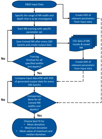
An implementation of the WGAN Algorithm was applied as the chosen algorithm, and an effort was made to change the network to be able to run on a GPU type Tesla P100, which decreases the training time required quite significantly. For the implementation of the WGAN scheme, two feedforward neural networks were applied. One as the discriminator, one as the generator. For the activation functions a ReLu function was used for all but the Output layer of the discriminator, which uses a Sigmoid function, since the result of this layer has to be a probability and Sigmoid functions give results between 0 and 1 [14]. For all of these implementations, the Pytorch library (version 1.5) was used [17]. The approach that was used to find the best possible NN for the input data is described inFigure 5as a flow chart, and in more detail in the text below.

Neural networks require hyperparameters to be fully functional. These are a set of parameters that are defined for the NN, before the training starts. The most important ones are the width and depth of the network, as explained above. These two hyperparameters are key for the training process, since they determine the number of neurons and the depth of the network. For each neuron, a weight exists as was explained above. By adapting the weights of the neurons for each processed batch the network actually learns the target distribution. Therefore, the number of neurons in a layer, as well as the amount of layers contributes immensely to the quality of the trained NN. Thus, width and depth were iteratively fitted in this study. This was done by training multiple NN with varying hyperparameter sets (especially for width and depth) which were changed iteratively in a looped approach. Therefore the parameter sets to be tested were defined before the training and then subsequently tested.

To train the MLA, a mini batch gradient descent procedure was utilized. In this procedure, the training data set is split into many, randomly generated, sub sets. The algorithm processes each mini batch separately and compares the cost function in relation to the current mini batch data. Subsequently, the network parameters are updated accordingly. This is done iterating over all mini batches, until the whole data set has been evaluated. This complete process is called an epoch. For the training in this study, a batch size of 64 was used, which is in line with batch sizes recommended in literature [18,19].

Other hyperparameters usually describe the learning rate of both, the generator network, as well as the discriminator network. However, the learning rate was automatically adapted, since an optimization algorithm called RMSProp was used for the back propagation. This optimization approach requires a low learning rate which is inherent to WGAN networks. Thus the influence of these parameters is negligible. Two important parameters are the clipping value and the dropout. Both variables represent values that are important in the NN to avoid overfitting and underfitting [20,21].

EBSD Input Data

Specify the range of NN width and

depth that is to be investigated

Save trained NN after every 200

Epochs and create output data

Training

finished for all

specified widths

and depths?

Start NN training with specific

parameter set

No

Yes

Create KDE of

relevant parameters

from Input data

CSV data of NN

results & saved

NN

Create KDE of

relevant parameters

from Input data

Compare Input data KDE with KDE

of generated output data for every

200 Epochs

Choose best fit by:

•

Mean deviation

•

Maximum deviation

•

Mean value of maximum and

median deviation

Comparison

done for all

trained NN

widths and

depths?

No

Yes

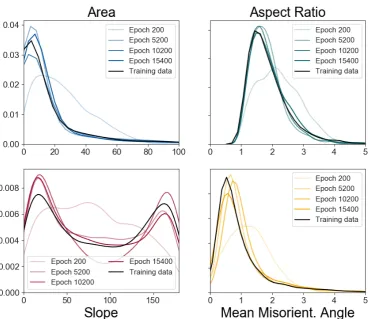
Figure 6.Development of the output of the NN over multiple epochs, compared to the input data. Epoch 15400 is the best fit for the applied input values.

only a defined number of epochs should be trained, since MLA are prone to overfitting in higher epochs.

After the training of all the different NN for multiple parameter sets is complete, the best fit needs to be found. To do so, a script was written, that creates a KDE of every microstructural parameter taken into account for the MLA training. Additionally, KDE of every taken snapshot are created of the same parameters, since this is the output of the generator network. Subsequently the fit between the input KDE and the synthetic data KDE are evaluated. This is done by investigating three types of deviation between the KDE of the real and synthetic data: The mean deviation, the maximum deviation and the mean value of both mean, and maximum deviation. All three are returned and can be checked by the user. Ideally, a NN snapshot can be chosen that shows the smallest deviation for all three values in comparison to the rest of the NN.

5. MLA results

After the training of the NN is completed, the network with the best results can be chosen. For this, the deviation of the KDE are utilized as described before. Since they show a significant development over the epochs, the best fit is the best averaged value, where most KDE curves fit the input KDE very well. The comparison of the best fit at epoch 15400 with the input data, as well as former epochs can be seen inFigure 6.

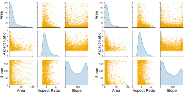
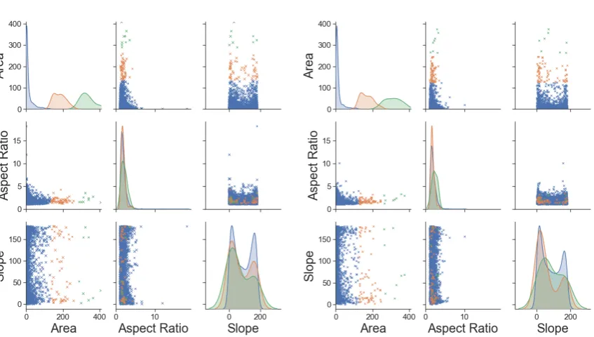
(a)Input data used for the training of the MLA (b)Synthetically created data

Figure 7.Comparison between the input data used for the training of the MLA and the output of the generator network at its best fit Epoch. Dependencies between the different microstructural parameters shown for a better evaluation of the results.

Figure 8.Development of the error of the output KDE compared to the input KDE over the course of the training. (Bild noch nicht Final)

input parameters at the best fit epoch very accurately. From the trained generator network data can then be extracted which is usable as input for e.g. RVE creation. The output of the NN follows the same format of the input. This means, that every parameter contained in the input data will be present in the output created by the MLA. Since the focus is the creation of input data that geometrically represents a grain (Figure 2), the main features to compare are area, aspect ration and slope. InFigure 7pairplots of both the input data and the synthetically generated output data are presented. On the diagonal, the KDE distributions are shown, while the other graphs show the respective parameters plotted against each other. From these pictures the compliance between real and synthetic grain data appears to be excellent.

6. Validation of the MLA results

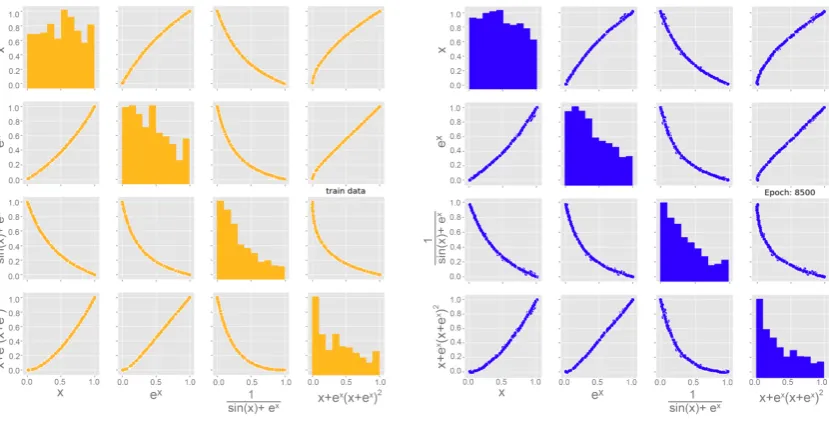
Only checking the appearance as well as the KDE of the plots however is not a sufficient validation of the NN output. Since the most important task of the machine learning algorithm was to represent the interdependencies of the microstructural parameters, a study was conducted to investigate, whether the applied algorithm is capable of handling interdependencies between input data. Therefore the MLA was trained on a specifically created data set with four parameters:

f1(x) =x (1)

f2(x) =ex (2)

f3(x) = 1

sin(x) +ex (3)

f4(x) =ex·(x+ex)2+x (4) Where x was generated from a uniform distribution. The other functions were arbitrarily chosen, with the criteria being that they all need to be dependent amongst each other. In this case equation 2) is dependent on equation 1), while 3) and 4) are dependent on both, 1) and 2). Thus all values were interconnected, and the implemented MLA was trained on this data set. The results, presented in Figure 9show, that the MLA is able to reproduce the input data very accurately. Both the distribution of each specific equation and the interdependencies as well show no significant deviation. It can therefore be assumed, that the implemented MLA is capable of representing any interdependencies that are present in the input data.

(a)Input data used for the training of the MLA (b)Synthetically created data Figure 9.Validation to see, whether the MLA is capable of representing the dependencies of its input data set, by applying multiple different interdependent equations. (Achsenbeschriftung muss noch angepasst werden)

(a)Clustering analysis of the input data (b)Clustering analysis of the synthetically created data Figure 10.Comparison between the clustering analysis of the input data and the generated output data. The area was divided into three equally sized sections for this analysis.

(which stand for grains with larger areas) is in a very similar position, but not the same. Most of the relevant points are at smaller aspect ratios and positioned near the 0◦or 180◦. No outliers are found in this analysis, which leads to the conclusion, that the interdependencies of the input data can be accurately portrayed.

7. Conclusions

This study presented a solution on how to generate input for microstructure modelling that is true to the real microstructure. Commonly, singular distribution functions are applied to describe the input for the microstructure model. However this study showed, that an approach like that is not suitable to describe any given microstructure in detail. Since there are at least three relevant parameters to each grain for each direction in space (area, aspect ratio, slope) all of these have to be represented accurately by statistic descriptions. The three aforementioned parameters are, in fact, all dependent on each other, where a relatively large grain tends to have smaller aspect ratios as well as a slope more parallel to the rolling direction.

To solve this challenge, this study applied a WGAN machine learning network to generate input data that represents all of the interdependencies. The results show, that the NN learns the distribution functions of the singular parameters very well. The generated output resembles the input quite accurately, while also representing the dependencies between the parameters. To validate these findings, a study was carried out to see, whether the implemented NN is able to recreate numerical relations between the different parameters. It was found, that the WGAN algorithm is capable of recreating the equations. To validate the results regarding the microstructural features, a clustering analysis showed, that the output data resembles the input data very accurately.

The implemented network in this study was trained on just one direction in space (rolling direction x sheet normal). To precisely describe any microstructure, however, it is necessary to show the influences of all three directions. Here the approach can be expanded. However, it is not an easy feat to generate statistically relevant information of the three dimensional structure from two dimensional pictures. A possible solution would be to simply train three networks, the question that remains unanswered is how the individual parameters of the three spatial directions relate. Answering this question will be a key focus in future work.

In comparison to other machine learning applications, this network was trained on a relatively small sample size. This was done deliberately, since in everyday research it isn’t always feasible to create a magnitude of EBSD pictures. The results from this study show therefore, that the applied concept works very accurately even on small sample sizes, where bigger data sets could only improve the quality of the output. Thus, this approach is suitable to be implemented even for small sample sizes and projects with smaller amounts of time and resources dedicated. Additionally, it is as easy as adding another column to and excel sheet, to train different parameters than the one used in this study or even add further parameters for the network to learn.

Funding: This research was funded by the Deutsche Forschungsgemeinschaft (DFG, German Research Foundation) – Projektnummer 278868966 – TRR 188

Acknowledgments: The support of this work by the Institute for Physical Metallurgy and Materials Physics (IMM) of RWTH Aachen and Carl Kusche is gratefully acknowledged, who provided the used EBSD pictures. Simulations were performed with computing resources granted by RWTH Aachen University under project rwth0463.

References

1. Pütz, F.; Shen, F.; Könemann, M.; Münstermann, S. The differences of damage initiation and accumulation of DP steels: a numerical and experimental analysis.

2. Lian, J.; Yang, H.; Vajragupta, N.; Münstermann, S.; Bleck, W. A method to quantitatively upscale the damage initiation of dual-phase steels under various stress states from microscale to macroscale. Computational Materials Science2014,94, 245–257. doi:10.1016/j.commatsci.2014.05.051.

3. Vajragupta, N.; Wechsuwanmanee, P.; Lian, J.; Sharaf, M.; Münstermann, S.; Ma, A.; Hartmaier, A.; Bleck, W. The modeling scheme to evaluate the influence of microstructure features on microcrack formation of DP-steel: The artificial microstructure model and its application to predict the strain hardening behavior. Computational Materials Science2014,94, 198–213. doi:10.1016/j.commatsci.2014.04.011.

4. Gitman, I.M.; Askes, H.; Sluys, L.J. Representative volume: Existence and size determination.Engineering Fracture Mechanics2007,74, 2518–2534. doi:10.1016/j.engfracmech.2006.12.021.

5. Bargmann, S.; Klusemann, B.; Markmann, J.; Schnabel, J.E.; Schneider, K.; Soyarslan, C.; Wilmers, J. Generation of 3D representative volume elements for heterogeneous materials: A review. Progress in Materials Science2018,96, 322–384. doi:10.1016/j.pmatsci.2018.02.003.

6. Ledl, T. Kernel Density Estimation: Theory and Application in Discriminant Analysis.Austrian Journal of Statistics2016,33, 267. doi:10.17713/ajs.v33i3.441.

7. Henrich, M.; Pütz, F.; Münstermann, S. A Novel Approach to Discrete Representative Volume Element Automation and Generation-DRAGen.Materials (Basel, Switzerland)2020,13. doi:10.3390/ma13081887. 8. Groeber, M.; Ghosh, S.; Uchic, M.D.; Dimiduk, D.M. A framework for automated analysis and simulation

of 3D polycrystalline microstructures.Part 1: Statistical characterization.Acta Materialia2008,56, 1257–1273. doi:10.1016/j.actamat.2007.11.041.

9. Groeber, M.; Ghosh, S.; Uchic, M.D.; Dimiduk, D.M. A framework for automated analysis and simulation of 3D polycrystalline microstructures. Part 2: Synthetic structure generation. Acta Materialia2008, 56, 1274–1287. doi:10.1016/j.actamat.2007.11.040.

11. Pütz, F.; Henrich, M.; Roth, A.; Könemann, M.; Münstermann, S. Reconstruction of Microstructural and Morphological Parameters for RVE Simulations with Machine Learning. Procedia Manufacturing2020, 47, 629–635.

12. Goodfellow, I.; Bengio, Y.; Courville, A.Deep Learning; MIT Press, 2016.

13. Sheehan, S.; Song, Y.S. Deep Learning for Population Genetic Inference. PLoS computational biology2016, 12, e1004845. doi:10.1371/journal.pcbi.1004845.

14. Goodfellow, I.; Pouget-Abadie, J.; Mirza, M.; Xu, B.; Warde-Farley, D.; Ozair, S.; Courville, A.; Bengio, Y. Generative Adversarial Nets. InAdvances in Neural Information Processing Systems 27; Ghahramani, Z.; Welling, M.; Cortes, C.; Lawrence, N.D.; Weinberger, K.Q., Eds.; Curran Associates, Inc, 2014; pp. 2672–2680.

15. Arjovsky, M.; Bottou, L. Towards Principled Methods for Training Generative Adversarial Networks. 16. Arjovsky, M.; Chintala, S.; Bottou, L. Wasserstein Generative Adversarial Networks. Proceedings of the

34th International Conference on Machine Learning; Precup, D.; Teh, Y.W., Eds.; PMLR: International Convention Centre, Sydney, Australia, 2017; Vol. 70,Proceedings of Machine Learning Research, pp. 214–223. 17. Paszke, A.; Gross, S.; Massa, F.; Lerer, A.; Bradbury, J.; Chanan, G.; Killeen, T.; Lin, Z.; Gimelshein, N.; Antiga, L.; Desmaison, A.; Kopf, A.; Yang, E.; DeVito, Z.; Raison, M.; Tejani, A.; Chilamkurthy, S.; Steiner, B.; Fang, L.; Bai, J.; Chintala, S. PyTorch: An Imperative Style, High-Performance Deep Learning Library. In Advances in Neural Information Processing Systems 32; Wallach, H.; Larochelle, H.; Beygelzimer, A.; Alché-Buc, F.d.; Fox, E.; Garnett, R., Eds.; Curran Associates, Inc, 2019; pp. 8024–8035.

18. Bengio, Y. Practical Recommendations for Gradient-Based Training of Deep Architectures. InNeural networks: Tricks of the trade; Montavon, G.; Orr, G.B.; Müller, K.R., Eds.; Springer: Heidelberg, op. 2012; Vol. 7700,Lecture Notes in Computer Science SL 1, Theoretical Computer Science and General Issues, pp. 437–478. doi:10.1007/978-3-642-35289-8$\backslash $textunderscore.

19. Masters, D.; Luschi, C. Revisiting Small Batch Training for Deep Neural Networks.

20. Pascanu, R.; Mikolov, T.; Bengio, Y. On the difficulty of training recurrent neural networks. International conference on machine learning, 2013, pp. 1310–1318.