Article
Persistent hot spot detection and characterisation
using SLSTR
Alexandre Caseiro1,∗ ID0000-0003-3188-3371, Gernot Rücker2, Joachim Tiemann2, David
Leimbach2, Eckehard Lorenz3, Olaf Frauenberger4, and Johannes W. Kaiser1
1 Max Planck Institute for Chemistry, Mainz, Germany
2 Zebris GbR, Munich, Germany
3 DLR, Berlin, Germany
4 DLR, Neusterlitz, Germany
* Correspondence: [email protected]; Tel.: +49-6131-305-4071
Academic Editor: name
Version June 29, 2018 submitted to Remote Sens.
Abstract:Gas flaring is a disposal process widely used in the oil extraction and processing industry. It 1
consists in the burning of unwanted gas at the tip of a stack and due to its thermal characteristic and 2
the thermal emission it is possible to observe and to quantify it from space. Spaceborne observations 3
allows us to collect information across regions and hence to provide a base for estimation of emissions 4
on global scale. We have successfully adapted the Visible Infrared Imaging Radiometer Suite (VIIRS) 5
Nightfire algorithm for the detection and characterisation of persistent hot spots, including gas flares, 6
to the Sea and Land Surface Temperature Radiometer (SLSTR) observations on-board the Sentinel-3 7
satellites. A hot event at temperatures typical of a gas flare will produce a local maximum in the 8
night-time readings of the shortwave and mid-infrared (SWIR and MIR) channels of SLSTR. The 9
SWIR band centered at 1.61µm is closest to the expected spectral radiance maximum and serves as the
10
primary detection band. The hot source is characterised in terms of temperature and area by fitting 11
the sum of two Planck curves, one for the hot source and another for the background, to the radiances 12
from all the available SWIR, MIR and thermal infra-red channels of SLSTR. The flaring radiative 13
power is calculated from the gas flare temperature and area. Our algorithm differs from the original 14
VIIRS Nightfire algorithm in three key aspects: (1) It uses a granule-based contextual thresholding to 15
detect hot pixels, being independent of the number of hot sources present and their intensity. (2) It 16
analyses entire clusters of hot source detections instead of individual pixels. This is arguably a more 17
comprehensive use of the available information. (3) The co-registration errors between hot source 18
clusters in the different spectral bands are calculated and corrected. This also contributes to the SLSTR 19
instrument validation. Cross-comparisons of the new gas flare characterisation with temporally close 20
observations by the higher resolution German FireBIRD TET-1 small satellite and with the Nightfire 21
product based on VIIRS on-board the Suomi-NPP satellite show general agreement for an individual 22
flaring site in Siberia and for several flaring regions around the world. Small systematic differences 23
to VIIRS Nightfire are nevertheless apparent. Based on the hot spot characterisation, gas flares can 24
be identified and flared gas volumes and pollutant emissions can be calculated with previously 25
published methods. 26
Keywords:Gas flaring; SLSTR 27
1. Introduction 28
Gas flaring (GF) is part of the upstream oil and gas industry processes as a means of disposing of 29
unwanted natural gas through high temperature oxidation at the tip of a stack. GF is a problem of local 30
2 of 30
and global concern. GF impacts the local environment [1] through: noise [2,3], visual pollution [4,5], 31
heat stress [4,6] and the emission of air pollutants like black carbon, polycyclic aromatic hydrocarbons, 32
volatile organic compounds and acid rain precursors [7–10]. Flaring produces greenhouse gases (GHG) 33
and black carbon as the main by-products of the combustion. In terms of the global GHG budget 34
gas flaring produced an estimated yearly average emission of 304 Tg CO2between 2003 and 2012, 35
representing 0.6% of the global carbon dioxide equivalent anthropogenic emissions [11]. Regarding 36
the short-lived climate forcer black carbon, GF may be of regional prime importance. GF has been 37
identified as the main input of black carbon in boreal regions [12,13], with implications for the albedo of 38
snow-covered surfaces, the earth’s radiative balance [14,15] and the Arctic amplification phenomenon 39
[16], being therefore of global relevance [17]. Again in the Arctic region, GF’s contribution to the NO2 40
concentrations is important, and has been increasing in the past decade [18]. 41
The information on flared volumes and emissions is sparse and methodologically inconsistent 42
due to technical difficulties and the lenient reporting requirements and guidelines of some jurisdictions. 43
Since GF creates a persistent or intermittent thermal signal, remote sensing offers the possibility of a 44
globally consistent and independent monitoring of flaring. Important applications of GF monitoring 45
are the estimation of the burnt gas volume in billion cubic metres (BCM) and the pollutant emissions 46
to the atmosphere. Such estimations have already been performed with the help of a conversion factor 47
that scales observed radiative energy release to BCM and emission factors that convert BCM into the 48
amount of different chemical smoke species [19]. The emission factors have been measured in-situ and 49
reported in the literature [20–22]. The conversion factor has been calculated as fraction of reported 50
BCM and the observed radiative energy in entire countries [19], at the regional scale or for individual 51
flares [23,24]. 52
The identification of flaring in the night-time observations in the visual and near infra-red 53
(Vis-NIR) spectral range [25,26] allowed for the first semi-automatic monitoring of flares from space 54
[27–29]. With the advent of vegetation fire detection products based on mid and thermal infrared 55
bands (MIR and TIR), flaring was highlighted as a main source of false alarms [30,31]. This feature was 56
exploited to study flaring [32,33] and later the additional evaluation of short-wave infrared (SWIR) 57
bands allowed for a more accurate detection [19,34–37], which is the current state-of-the-art. 58
Algorithms exploiting the IR part of the spectrum for flare detection and characterisation have 59
been developed for a number of sensors. Casadio et al. [35] considered the radiances at four 60
wavelengths (in the SWIR, MIR and TIR bands of (A)ATSR, (Advanced) Along Track Scanning 61
Radiometer) to be a linear combination of black body radiances from two areas with different 62
temperatures within the satellite pixel footprint (actively flaming and background). Besides using 63
the 1.61µm channel for the detection, the authors also discriminated between persistent (at least 4
64
detections a year at a given location) and non-persisten signals, and attributed persistent detections 65
to gas flaring. Elvidgeet al. [36] developed the Nightfire algorithm, in which a Planck curve is 66
fitted to the night-time Vis-IR measurements of the Visible Infrared Imaging Radiometer Suite 67
instrument (VIIRS, on-board the Suomi-National Polar Partnership satellite) to retrieve the hot 68
spot temperature. They considered an emission scaling factor to estimate the flare size. The 69
methodology was further developed into a dual Planck curve fitting (for the background and 70
the flare) to the observations in five bands (NIR, SWIR and MIR) of VIIRS [19]. It was used to 71
retrieve information on the global distribution and characteristics of gas flaring and the results 72
are made public by NOAA’s National Centre for Environmental Information as daily global fields 73
(https://ngdc.noaa.gov/eog/viirs/download_viirs_fire.html). It was later demonstrated that the 74
SWIR radiance could be used by itself to estimate the flaring radiative power [38]. Gas flaring in 75
Africa was also monitored using Landsat [37] and MODIS [23] imagery. The former algorithm used 76
a thresholds series for the NIR, SWIR and TIR bands, and the latter used a combination of a fixed 77
threshold and spatial filtering. The BIRD algorithm was developed to apply the bi-specral method [39] 78
to MIR and TIR data from the Hot Spot Recognition System (HSRS) instrument on board the bi-spectral 79
Infrared Detection (BIRD) Experimental Small Satellite (2001-–04) [40–42]. It was designed to retrieve 80
Preprints (www.preprints.org) | NOT PEER-REVIEWED | Posted: 24 June 2018 doi:10.20944/preprints201805.0020.v2
effective temperature, effective area and effective radiative power of sub-pixel hot sources, namely 81
fires [43,44]. The methodology was later ported to the successor FireBIRD mission, with a similar 82
sensor in IR and a modified Vis-NIR payload on board of the TET-1 (Technologieerprobungsträger-1) 83
spacecraft [45]. 84
The Sea and Land Surface Temperature Radiometer (SLSTR) instrument on board ESA’s Sentinel-3 85
features night-time observations in two SWIR (S5: 1.61µm and S6: 2.25µm), one MIR (S7: 3.74µm)
86
and two TIR bands (S8: 10.85µm and S9: 12.0µm). The instrument also measures in two fire-dedicated
87
bands (F1: 3.74µm and F2:10.85µm) with the same central wavelength and band width as S7 and
88
S8, but extended dynamical ranges to prevent saturation over active fires. [46] The distribution of 89
the SLSTR spectral channels with SWIR, MIR and 2 channels in TIR should allow for the detection 90
and characterisation of GF and other hot spots via the SWIR detection and dual Planck curve fitting 91
methodology. Compared to VIIRS, SLSTR is observing in one additional SWIR channel at night-time 92
and it has better signal-to-noise requirements [47,48]. SLSTR can therefore be expected to detect even 93
smaller and cooler hot targets than VIIRS. However, SLSTR is missing the observations in the visible 94
spectral range,i.e. VIIRS’ DNB channel, which may make the temperature retrieval less accurate. 95
Furthermore, the long-term commitment of the EU Copernicus programme, which funds the Sentinel 96
satellites, would warrant data availability well into the 2030s. 97
In this paper, we present a new algorithm for the detection and characterisation of persistent hot 98
spots, including gas flares, detection and characterization from SLSTR observations and apply it to 99
actual SLSTR data. Section2presents the data used. Section3describes the developed methodology 100
in detail. In Section4we present the results of the application of the newly developed algorithm at the 101
regional level in four regions of interest (West Africa, The North and Caspian Seas and the Persian 102
Gulf) and evaluate our methodology against the VIIRS Nightfire product. The performance of our 103
algorithm is further evaluated against VIIRS Nightfire and retrievals based on HSRS on-board the 104
German small satellite TET-1 at the level of a single gas flaring site on the Yamal peninsula, Northern 105
Siberia. Finally, in Section5we present our conclusions. 106
2. Data 107
SLSTR Level 1b version 2 products obtained from the ESA’s Sentinel Expert User’s Hub in January 108
2017 were used for this work. The downloaded products were selected using a geographic criterion 109
(four regions of interest: West Africa, the Caspian and the North Seas and the Persian Gulf) and a 110
time of day criteria (only night-time acquisitions). The products were sampled in the second half of 111
2016. For the SWIR bands (S5 and S6), the data available in the product are top of the atmosphere 112
(TOA) radiances, while for the MIR (S7 and F1) and TIR (S8, S9 and F2) bands, the available data 113
are brightness temperatures. The latter were converted back to TOA radiances using lookup tables 114
provided by the European Space Agency. 115
FireBird TET-1 level-2 co-registered data of TET-1 night time acquisition mode (only MIR and TIR 116
bands at 170 m spatial resolution) were obtained for near coincident or temporally close SLSTR and 117
TET-1 observations during polar night conditions in 2016/17 over the Yamal peninsula and other areas 118
in Northern Siberia. Due to solar light contamination, only data North of about 70◦latitude could be 119
used, which excluded the other regions. Probably due to the extremely cold background, the standard 120
level-2 fire processor of FireBird [45] failed to identify valid background pixels, and thus did not detect 121
any hot clusters. The co-registered data were therefore reprocessed with the BIRD night-time algorithm 122
[42] which was adapted to the spatial resolution of TET-1 and the cold background. The algorithm 123
for fire detection and characterisation output includes an estimate of the fire area together with their 124
uncertainties [42] which were used for comparison with the temporally close SLSTR retrievals. The 125
BIRD algorithm artificially sets the upper temperature bounds to 1500 K to avoid unrealistically high 126
bi-spectral retrievals in the case of overestimations of the TIR background radiance. This limit was 127
4 of 30
Table 1.Comparison between the used sensors.
HSRS VIIRS SLSTR
on TET-1 on Suomi-NPP on Sentinel-3A
Start of operation 2013 2011 2016
Orbit Sun synchronous Sun synchronous Sun synchronous
altitude (km) 445 834 814.5
Vis-NIR bands DNB: 0.5 – 0.9
(µm) M7: 0.85 – 0.89
M8: 1.23 – 1.25 SWIR bands
M10: 1.58 – 1.64 S5: 1.58 – 1.65
(µm) S6: 2.23 – 2.28
Infrared
MIR: 3.40 – 4.20 TIR: 8.50 – 9.30
M12: 3.55 – 3.93 S7, F1: 3.55 – 3.93
bands M13: 3.97 – 4.13 S8: 10.40 – 11.30
(µm) M15: 10.26 – 11.26 S9, F2: 11.50 – 12.50
Ground
IR-bands: 170 M-bands: 750 S4–S6: 500
resolution (m) S7–S9, F1–F2: 1000
Swath (km) IR: 178 3040 1420
Table 2.Data used in this study. The number of VIIRS products was derived from the VIIRS Nightfire dataset from NOAA, corresponding to the products which exhibited detections co-located in space and time.
Sensor Region Sampling dates n
Regional study
SLSTR
North Sea 17/11 – 18/12/2016 189 Caspian Sea 17/11 – 20/12/2016 99 Persian Gulf 17/11 – 31/12/2016 153
West Africa 25/07 – 29/09/2016 364
VIIRS (Nightfire) Global 2016 587
Single site study SLSTR Yamal peninsula 15/12/2016 – 02/01/2017 43
VIIRS (Nightfire) 6
HSRS 12
VIIRS Nightfire data [36] were downloaded from the NOAA website . No further processing was 129
applied to this dataset. 130
Table1summarizes the specifications of the used sensors, while Table2summarizes the data 131
used. 132
3. Methodology 133
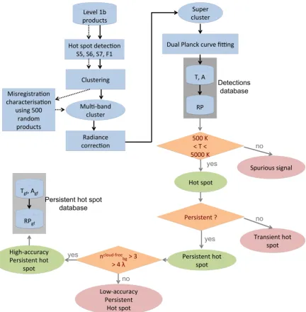
A general flowchart of the developed methodology is shown in Figure 1. The individual 134
processing steps are described in the following sections. 135
3.1. Detection 136
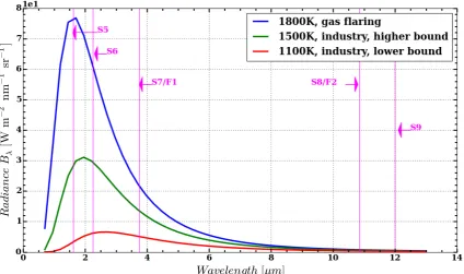
The SLSTR SWIR channels S5 and S6 capture the peak radiation of typical industrial (1100 – 1500 137
K) and gas flaring temperatures (around 1800 K) [19,49,50] as given by the Planck equation (Figure2). 138
The ability of SLSTR to detect hot spots in the SWIR and MIR bands was evaluated according to the 139
instrument’s requirements and is shown in Figure3and compared to VIIRS. In the 1.6µm channel,
140
SLSTR is expected to perform similarly as VIIRS. VIIRS does not record in the 2.25µm channel at night.
141
In the 3.7µm channels, VIIRS shows more sensitivity to cooler hot spots but SLSTR is, thanks to the
142
extended dynamic range of F1 which complements S7, theoretically able to quantify larger and hotter 143
hot spots. 144
Remote detection of gas flares with space-borne SWIR observations has been using a priori fixed thresholds on one or several bands [34,35,37] or determining the threshold based on the pixel’s surroundings, i.e. contextual thresholding [19,23,36]. In the present work, we use contextual thresholding. Due to the representation of the observations as digital numbers (DN) in the satellite
Preprints (www.preprints.org) | NOT PEER-REVIEWED | Posted: 24 June 2018 doi:10.20944/preprints201805.0020.v2
Figure 1.General algorithm flowchart for the detection of persistent hot spots and their characterisation: temperature (T), area (A) and radiative power (RP). The dotted line represents the one-time misregistration determination. The parameterization was then used when building the multi-band cluster. ncloudbg −f ree > 3 represents at least three cloud-free pixels in the background. >4λmeans
6 of 30
Figure 2.Planck curves for typical industrial processes and gas flaring temperatures, together with SLSTR SWIR (S5 and S6), MIR (S7 and F1) and TIR (S8, S9 and F2) channels. Temperatures of 1100 K and 1500 K represent, roughly, the lower and upper bounds of the operating temperatures of blast furnaces. 1800 K is a typical gas flaring temperature.
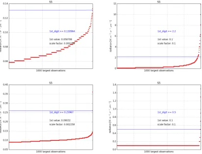
downlink, all radiance values within a single scene are multiples of a fixed radiance value, i.e. a step sizes fλ. This is clearly visible in the top-left panel of Figure4. For each scene and channel, we
determine the threshold radianceBthreshold
λ as the lowest multiple of the step size that is not reported
for any pixel:
Bthresholdλ =min{Blargestλ,i |Bλlargest,i −Blargestλ,i−1 >s fλ} (1)
whereBλlargest={Bλ,−999, ...,Bλ,0|Bλ,i ≤Bλ,i+1}is the ordered set of the 1000 largest radiances in the 145
granule (typically SWIR bands: 2400×3000 pixels per granule, MIR and TIR bands: 1200×1500 146
pixels per granule), ands fλis the scale factor for the product and that band, which is calculated from
147
the smallest interval between the recorded values. Radiance values below the threshold are interpreted 148
as smoothly varying background plus "typical” noise, while radiance values above the threshold are 149
interpreted as potential hot spot detections and are processed further. 150
We have tested several other approaches on the ordered set of the radiances of a product: 151
• The cut-off value was set as the lowest radiance which produced two statistically distinct groups 152
(using the Mann-Whitney-Wilcoxon U-test). This approach failed to produce thresholds for the 153
majority of products. 154
• The cut-off value was the lowest radiance which was not included within the confidence interval 155
of the linear regression of the previous points. This methodology lead to the inclusion of 156
irrealistically low radiance pixels as hot pixels and the subsequent production of extremely large 157
clusters. 158
• Also based on the linear regression, we examined where the slope changed significantly and 159
whether that point could be used as a threshold. This was highly dependent on the assumptions 160
on the linear regression and considered as non robust. 161
• Otsu’s method [52] produced large thresholds and therefore left out real hot spots. 162
Preprints (www.preprints.org) | NOT PEER-REVIEWED | Posted: 24 June 2018 doi:10.20944/preprints201805.0020.v2
Figure 3. Isoradiance lines for the noise (SWIR bands S5 and S6 and MIR bands S7 and F1) and saturation levels (MIR bands S7 and F1) for SLSTR and noise and saturation for the SWIR and MIR bands (M10, M12 and M13) of VIIRS used in the Nightfire algorithm. The SLSTR noise levels were computed using the End-of-Life noise-equivalent differential reflectance (S5 and S6) and noise-equivalent differential temperature levels (S7 and F1) [47] and were 1.5×10⁻², 8.4×10⁻³, 2.6×10⁻⁴and 2.1×10⁻¹W m−2µm−1sr−1for S5, S6, S7 and F1 respectively. A reflectance of 30% as
8 of 30
Figure 4.Four examples of thresholding for the S5 band. The horizontal line marks the threshold value. The threshold is set contextually as the lowest radiance value whose difference to the closest inferior radiance value is larger than the scale factor.
• An iterative clustering method which minimized differences between radiances of data points 163
within two clusters also lead to large thresholds. 164
• Based on the fact that the night-time background is rather homogenous, the variance of the 165
radiances of the product should be increased strongly by hot spots, while the background pixels 166
should have a small variance. This approach was very sensitive on the a priori explained variance 167
expected and was therefore abandoned. 168
The selected approach was the most robust, identifying hot pixels in different contexts with low 169
variation between different products. This approach captures hot pixels when there is a gradual or 170
an abrupt increase (upper and lower plots of Figure4, respectively). While not fixed, and therefore 171
adaptable to product-specific conditions, this contextual methodology is not statistical and therefore 172
not directly sensitive to the number of hot events sampled and their intensity. 173
At the end of this step, a collection ofihot pixels are registered, for each of the four SWIR and 174
MIR bands, with the following information: 175
• hot pixel location (xi,yi) as pixel index pair 176
• radianceBλ,iinWm
−2µm−1sr−1 177
• areaAλ,i inm2(the the pixel length on thexandyaxis is computed as average of the ground 178
distance between the pixel and its direct neighbours in those axes). 179
Preprints (www.preprints.org) | NOT PEER-REVIEWED | Posted: 24 June 2018 doi:10.20944/preprints201805.0020.v2
3.2. Clustering 180
The clustering of contiguous hot pixels is necessary because the signal of a single hot spot may 181
influence more than one pixel [33,53]. It may also be the case that a single hot spot is detected in two 182
or more adjacent pixels. [23,37] Indeed, in the case of flaring a facility may comprise arrays of many 183
flares with sizes of up to several hundred metres, while individual stations are several kilometres apart. 184
The misregistration between SLSTR channels is not an issue here because the IR bands are treated 185
independently up to the step right before the characterisation (see section3.6). 186
A cluster is defined as a set of hot pixels which are adjacent spacially. A cluster may comprise 187
only one pixel if none of its adjacent pixels are hot. 188
A background area is defined as extending two pixels beyond the cluster’s limits in any direction, 189
including diagonally and excluding the cluster of hot pixel(s) itself . For each single pixeliof then 190
cluster’s pixels, the radianceBλ,iand areaAλ,iare registered. Likewise, for each single pixeljof them
191
background pixels,Bλ,jandAλ,jare registered. 192
For each cluster, the following quantities are then computed: the average radiance and its 193
standard deviation in[Wm−2µm−1sr−1], the average background radiance and its standard deviation
194
in[Wm−2µm−1sr−1], the cluster area in[m2], its x-position as across-track index and y-position as
195
along-track index, and the number of cloud-flagged pixels (using the standard SLSTR cloud product) 196
for both the cluster and the background. 197
3.3. Misregistration characterisation 198
A hot event at temperatures typical of a gas flare, a steel mill or an iron smelter, will produce a 199
local maximum in the SWIR and MIR channels (see Figure2), which will be translated into a cluster in 200
those bands. The MIR fire channels S7/F1 of SLSTR have been designed with a different footprint size 201
and position than the corresponding SWIR channels. Because of these differences the clusters in the 202
different bands cannot be spatially superimposed. 203
We determine the misregistration of channels S6, S7 and F1 relative to channel S5 by assuming 204
that the majority of hot spots are isolated point sources: For each hot spot cluster in S6, S7 and F1, taken 205
from a random set of 500 SLSTR scenes, the closest S5 cluster is found. For each pair, the distances of 206
the cluster centres in along-track and across-track directions are calculated in coordinates of product 207
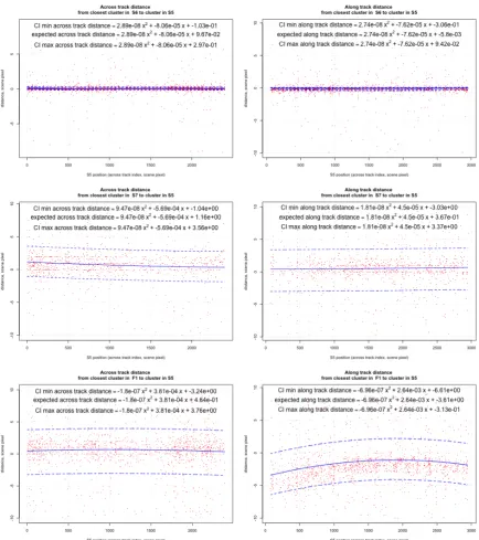
image grid indeces. These distances are plotted over the across-track pixel position in Figure5. 208
A systematic dependency on the across-track position is obvious in several of the plots. We, 209
therefore, fit parabolas to the data. They represent our best estimate of the misregistration between S5 210
and S6 resp. S7 resp. F1. The fitted parameters are given in Figure5. In order to determine confidence 211
intervals for the misregistration estimates, the fitted parabolas are shifted vertically such that 10% of 212
the data points are below resp. above. 213
3.4. Misregistration correction: building multi-band clusters 214
Multi-band clustersChotspotare subsequently constructed. They consist of the single-band clusters Cλwithλin S5, S6, S7 and F1 that observe the same hot source. The SWIR clusterCS5 is used as
reference. Then those clusters from the remaining bands (Cλwithλin S6, S7 and F1) that are closest to
after correction of the misregistration are added. In doing so, only clusters in the confidence intervals are considered:
min{d|(xλmin≤ |xS5−xλ| ≤x
max
λ ∧y
min
λ ≤ |yS5−yλ| ≤y
max
λ )} →C
hotspot
λ =Cλ (2)
where 215
Cλis any of theλ-band clusters (λin S6, S7 and F1),
216
Chotspotλ is theλ-band cluster within the multi-band clusterChotspot(λin S6, S7 and F1),
217
d= ((xλ−xavgλ )2+ (y
λ−y
avg
λ )
2)12 is the distance betweenC
λand the parameterised misregistration
218
position for the bandλ,
10 of 30
Figure 5.Parameterizations of the distances between a cluster in S5 and the closest cluster in S6, S7 and F1 as a function of the scan index. The solid line shows the best fit (second order polynomial). The dashed lines are parallel to the best fit so that 10% of the points are above resp. below. They represent the confidence interval.
Preprints (www.preprints.org) | NOT PEER-REVIEWED | Posted: 24 June 2018 doi:10.20944/preprints201805.0020.v2
xS5andyS5are the across track and along track position of the S5 reference clusterChotspotS5 , 220
xλandyλare the across track and along track position ofCλ,
221
xavgλ ,xminλ andxmaxλ are the average, minimum and maximum distances in the across track axis given 222
by the misregistration parameterisation as a function of the reference cluster across track positionxS5, 223
yavgλ ,yminλ andymaxλ are the average, minimum and maximum distances in the along track axis given by 224
the misregistration parameterisation as a function of the reference cluster across track positionyS5. 225
For the TIR bands S8, S9 and F2, the flaring high-temperature event is not expected to impact the 226
radiance (Figure2). The average radiance for each TIR band 2 pixels around the reference S5 cluster 227
position is then associated to the multi-band cluster. 228
3.5. Radiance corrections 229
The SWIR radiances in S5 and S6 exhibit a systematic overestimation of 11 and 20%, respectively. 230
[54] Following recommendations by ESA, all values in the SWIR bands were corrected accordingly. 231
This correction needs to be verified and possibly updated for future versions of SLSTR products. 232
After building the multi-band clusters, the MIR S7 channel is checked for saturation. If the S7 233
radiance is above the upper limit of the linearity range (0.56Wm−2µm−1sr−1, corresponding to a
234
brightness temperature of 306K) in any of the hot pixels within the cluster, then it is discarded. If the 235
S7 cluster is discarded or not present, the F1 cluster is used. The F1 band is a fire dedicated channel of 236
SLSTR which measures at the same wavelength as the S7 channel, but with a larger dynamic range 237
and lower sensitivity. Only F1 clusters where all of the pixels have a brightness temperature within the 238
range 300–480 K are considered, as this is the range where the Level 1 quantification is accurate. 239
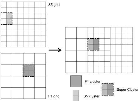
3.6. Super Cluster definition 240
The areas of the individual clusters in the SWIR and MIR bands within a multi-band cluster may 241
vary. To overcome this, hypothetical super clusters, with perfect coregistration and identical footprint 242
areas in all bands, are built. The largest of the individual band clusters’ areasAλis chosen as area
243
Aclusterof the super cluster (Figure6). 244
For each band’s clusterCλhotspotwithin a multi-band clusterChotspot, the observed cluster radiance Bobs
λ is calculated as area-weighted average of the observed radiances of the cluster and the background:
Bobsλ = Bλ×Aλ+B
bg
λ ×(Acluster−Aλ)
Acluster
(3)
It is assumed that the background radianceBbgλ is constant in the vicinity of the cluster. For the 245
TIR bands (S8, S9 and F2) the weighting is not necessary as the hot spot signal is not expected to be 246
distinguishable from the background in that spectral region and the average radiance of background 247
and cluster, is used. 248
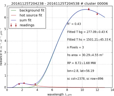
3.7. Planck curve fitting 249
In order to determine the temperature and the area of the flaring event, the sum of two Planck 250
curves is fitted to the radiance data of the multiband cluster, as established by Elvidgeet al.[19]. The 251
two Planck curves represent the two contributors for the IR radiance measured by the sensor at night, 252
i.e. the flaring event and the background, each weighted by its respective relative area: 253
Bobsλ =! B(λ,Tbg)×(1−
Ahotspot Acluster
) +B(λ,Thotspot)×
Ahotspot Acluster
(4)
B(λ,T) = 2hc
2
λ5 1
eλkThc −1
12 of 30
Figure 6.Super cluster creation.
Preprints (www.preprints.org) | NOT PEER-REVIEWED | Posted: 24 June 2018 doi:10.20944/preprints201805.0020.v2
Figure 7.An example of the temperature and area retrieval by dual Planck curve fitting.
whereB(λ,Thotspot)andB(λ,Tbg)are the modelled hot spot and background radiance, respectively, 254
according to Planck’s law.Ahotspotis the modelled flame area[m2]. 255
TheBobsλ values , obtained from the Super Cluster (see section3.6), are approximated by fitting 256
the parametersTbg,ThotspotandAhotspotvia the least squares methodology. The standard deviation of 257
the background radiancesσλbgis used in the fitting as standard deviation of the cluster radiances. The
258
algorithm computes uncertainties for both the temperature and the area. 259
3.8. Radiative power 260
The radiative power (RP) of the hot source may then be computed using the Stefan-Boltzmann 261
equation and assuming a perfect emissivity (in W): 262
RPhotspot =Ahotspot×σSB×Thotspot4 (6) whereσSBis the Stefan-Boltzmann constant (5.670373×10⁻⁸Wm−2K−4). The respective uncertainty is 263
computed by propagation of errors. 264
Elvidgeet al.[19] used the VIIRS M10 band as a primary band for the detection of gas flares 265
and found that "there is a strongly coherent linear relationship between top of the atmosphere and 266
atmospherically corrected RH [radiant heat]". The authors thus conducted their work with the 267
uncorrected TOA radiances. Since the S5 band of SLSTR is within the same clear atmospheric window, 268
14 of 30
4. Results 270
4.1. Regional study: 4 flaring regions 271
The described algorithm was applied to observations in the four regions of West Africa, the North 272
sea, the Caspian sea and the Persian gulf, cf. Table2. 273
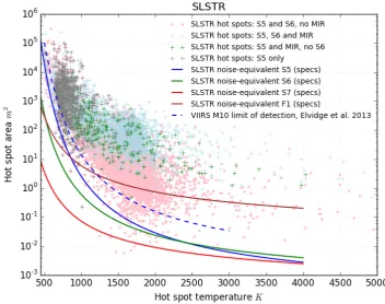
4.1.1. Detection thresholds 274
Figure8shows the relationship between the retrieved temperature and area of hot spots detected 275
by SLSTR and compares it with the noise-equivalent radiance levels for the detection bands (S5, S6, 276
S7 and F1) and with the limit of detection derived for VIIRS Nightfire [36]. The cloud of points 277
generally follows the M10 detection limit derived by Elvidgeet al.[36], but also expands slightly to 278
lower threshold values in the regions of typical industrial temperatures (around 1000K) and gas flaring 279
(1500–2000K). 280
Hot spots detected in the S5 channel only (grey crosses in Figure8) represent 5% of all the hot 281
spots within the study regions. They exhibit temperatures in the lowest end (600–1000K) of the range 282
of retrieved temperatures and areas in the upper end (102–105) of the range of retrieved areas. These 283
values are highly uncertain because only one constraint exists in the SWIR and MIR range so that 284
the TIR radiances are expected to be overfitted. The retrievals are thus treated as "low-accuracy" (see 285
Section4.1.4). Clusters detected in the MIR (green and blue crosses in Figure8) represent 28% of 286
all the hot spots within the study regions (3% S5 and MIR and 25% in S5, S6 and MIR). The lower 287
limit of the cloud follows an isoradiance line that represents a larger radiance value (approximately 288
5W m−2sr−1µm−1) than the noise-equivalent for S7 or F1 from the instruments specifications. We
289
attribute this to the larger variability of the background in the MIR. Hot spots detected in both SWIR 290
channels (S5 and S6) but not in the MIR channels (pink points in Figure8) make up the most of the 291
detections (67%). Hot spots in the region below the M10 limit of detection (blue dashed line) as derived 292
by Elvidgeet al.[36] were detected in both SWIR channels. They are mostly in the expected range 293
for gas flares (1300–2000K [19]). This suggest some capability, thanks to the availability of both SWIR 294
channels, to detect smaller gas flares than those detected by VIIRS. SLSTR can also characterise the 295
smaller gas flares more effectively using the Planck curve fitting method. 296
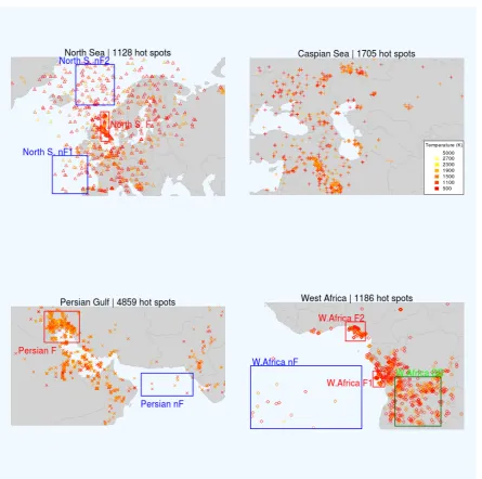
4.1.2. Temperature and area retrievals 297
Figure9shows the hot spot detections of SLSTR with temperatures in the range [500 K, 5000 298
K], which we consider to relate to actual hot spots on the ground . The methodology identifies hot 299
spots in regions where flaring is known to occur (e.g. the North Sea oil fields, the mouths of the 300
Congo and Niger rivers, the Persian Gulf and the Tigris and Euphrates rivers valleys). Figure10shows 301
the temperature distributions in nine specific areas: four areas with know gas flaring, one area with 302
biomass burning and four areas without any known hot objects. Hot spots detected offshore where 303
no oil extraction activities are present show a clearly lower temperatures than for the other study 304
regions. Hot spots were also detected in the plateau of central Angola and the Southern D. R. Congo. 305
The intermediate temperatures retrieved in those regions indicate the presence of biomass burning. 306
Observing fire temperature on a global scale, even only at night-time, is complementary to the widely 307
used burnt area and fire radiative power observations and has great potential for reducing errors in 308
the current vegetation fire emission datasets. 309
Hot spot characteristics evaluated from space could be dependent on the viewing angle. This 310
was shown to be relevant for VIIRS [19]. However, SLSTR has a narrower range of viewing angles 311
and the effect is not expected to be as pronounced. Since we fit an unconstrained Planck curve, this 312
effect would be noticed in both the retrieved temperature and area. We therefore present the retrieved 313
hot spot radiative power variation dependending on the across track index in Figure11. There is no 314
apparent effect. 315
Preprints (www.preprints.org) | NOT PEER-REVIEWED | Posted: 24 June 2018 doi:10.20944/preprints201805.0020.v2
16 of 30
Figure 9.Maps of the hot spots within the test regions. The rectangles represent the 9 study areas (red for flaring, green for biomass burning, blue for non-flaring)
Preprints (www.preprints.org) | NOT PEER-REVIEWED | Posted: 24 June 2018 doi:10.20944/preprints201805.0020.v2
Figure 10. Temperature retrievals distribution for the hot spots within each study area defined in Figure9.
4.1.3. Persistence 316
Hot or bright events that can be observed from space in the IR part of the spectrum at night 317
include gas flares, wildfires, auroras, industry (e.g.steel mills) and volcanoes. [34,36] Noise and an 318
increased exposition of the sensor to radiation due to the South Atlantic Anomaly may also generate 319
spurious hot spots. [19,34] It is possible to discriminate between these events based on retrieved 320
characteristics, such as the temperature. [19,55] In the present work, we opt for an analysis of the 321
persistence of the signal at the location of a given hot spot as it has been used previously to filter out 322
noise and ephemeral phenomena [19,34]. 323
We base the definition of our criterion on the work of Casadioet al.[34], who used a threshold of 324
at least 4 detections a year for (A)ATSR, the heritage instrument of SLSTR. Since the swath of (A)ATSR 325
is roughly one third of SLSTR’s, the criterion would correspond to 12 times a year for SLSTR. The 326
sampling period is roughly 2 months, corresponding to 2 observations within that period. This was 327
raised to 3 in order to filter out noise. 328
Although not suitable for a thorough analysis due to the short sampling period, the persistent hot 329
spots (at least 3 detections within a spatial accuracy of±0.02 degrees in longitude and latitude over 330
the sampling period) mainly correspond to locations within known flaring regions (see Figure12). In 331
future works where this methodology will be used on data from longer periods, this threshold might 332
need to be raised or otherwise adapted. For known interferences, persistent or semi-persistent hot 333
sources such as volcanoes, the use of a mask will also be useful. 334
The persistent locations thus derived were compared with high resolution imagery (Google Earth, 335
for the Caspian Sea test region) in order to check for the existence of a hot spot: at 96 (65%) of the 148 336
persistent hot spot locations a gas flare was visible, 34 (23%) locations were offshore or onshore but 337
lacking sufficient resolution, 12 (8%) were onshore locations without an industrial area nor a visible 338
gas flare nearby and 6 (4%) were at an industrial site without a visible flare. 339
4.1.4. Selection of persistent hot spots and radiative power computations 340
In order to filter low-quality determinations, cloud cover and overfitting were considered. 341
Clouds may interfere with the amount of radiation measured by the SLSTR instrument, in turn 342
interfering with the temperature, area and radiative power retrievals. However, simply discarding 343
cloudy pixels could incur a large omission error since pixels containing gas flares are frequently marked 344
18 of 30
Figure 11.Retrieved radiative power for hot spots as a function of the across track index (ATI).
Preprints (www.preprints.org) | NOT PEER-REVIEWED | Posted: 24 June 2018 doi:10.20944/preprints201805.0020.v2
20 of 30
Table 3.Summary of the detections based on SLSTR and spatial comparison with VIIRS Nightfire.
North Sea Caspian Sea Persian Gulf West Africa SLSTR
hot spots 1128 1705 4859 1186
persistent hot spots 467 1182 4032 385
high-accuracy persistent hot spots 203 874 3096 15
persistent locations 72 148 359 57
persistent locations detected by VIIRS 71 148 359 57
analyse the cloudiness of the background, as defined in section3.2, and discard only observations with 346
less than 3 cloud-free background pixels. 347
In order to avoid too much dependence on the TIR channels, which are not affected by small hot 348
sources with the temperature of gas flares, we discard persistent hot spots for which no clusters were 349
detected in S6, S7 and F1. In the work of Elvidgeet al.[19], signals detected in the 1.6µm channel only
350
are not quantitatively evaluated and information from nearby hot spots is used. Although we compute 351
the hot spot temperature and fraction area and the background temperature with the dual Planck 352
curve fitting (section3.7) using data from the super cluster (S5 and TIR channel, section3.6), we opt to 353
discard those results (clustered in a low temperature/large area region, Figure8) and to not assume 354
any characteristics for that particular detection. Since these detections are only 5% of the total hot spot 355
persistent detections, we assume that they do not significantly influence hot spots characterization 356
within the study regions. 357
Figure13shows the distributions of the retrieved temperature, area and radiative power for 358
detections that have been filtered with the persistence, cloud cover and S6/S7/F7 availability criteria 359
described above. We will label these "high-accuracy persistent" below. A range of temperatures 360
around 1800 K can be considered as characteristic for flaring [19,36], and the distributions of the 361
high-accuracy persistent hot spots fall mostly within the expected range for gas flares, but observations 362
in the 500–1500 K temperature range are also important. The retrieved temperatures show a clearly 363
unimodal distribution approximately centered at 1600 K for the Persian Gulf and the Caspian Sea test 364
regions. For the North Sea test region, the distribution is bi-modal, with modes around 1000 K and 365
1600 K. While the latter is probably associated with gas flaring, the former is more likely associated 366
with industry (see Figure12, the colder persistent detections are onshore.). [19] There were very few 367
high-accuracy persistent hot spots for the West Africa test region due to unfavourable cloud conditions. 368
4.1.5. Comparison with VIIRS Nightfire 369
The SLSTR hot spot at persistent locations were compared to the VIIRS Nightfire data for a 370
same time period and a roughly similar area. The VIIRS Nightfire results were subject to the same 371
spatial persistency analysis as the SLSTR data (3 times within a spatial accuracy of 0.02 degrees in 372
longitude and latitude). VIIRS detects more gas flaring locations than SLSTR, which can be traced 373
back to its wider swath (3040 km against 1420 km), and thus a shorter revisit time. Another reason 374
for the larger number of detections by VIIRS is that the Nightfire algorithm processes single pixels, 375
selected as the local maxima of pixels above the threshold, the method here aggregates contiguous hot 376
pixels into clusters. Despite these differences , all but one persistent locations detected by SLSTR were 377
also detected by VIIRS (Table3). The VIIRS Nightfire algorithm produces a slightly larger fraction 378
of detections in the 1.6µm channel only (7% for Nightfire against 5% for the present work). But
379
when considering Nightfire detections in the 1.6µm and visible (0.5-0.9µm, Day-Night Band, DNB)
380
channels, the fraction is very important: 55%, as is the fraction of SLSTR hot spots detected in both 381
SWIR channels only (67%). The MIR channels, both of VIIRS and SLSTR, produce less detections than 382
the SWIR channels. We interprete this as a larger variability of the background in the MIR region, as 383
well as a lower sensitivity to high temperature sources (Figure2). 384
Preprints (www.preprints.org) | NOT PEER-REVIEWED | Posted: 24 June 2018 doi:10.20944/preprints201805.0020.v2
22 of 30
Table 4. Summary of the detections at the Bovanenkovo gas and condensates field in the Yamal Peninsula, Siberia.
SLSTR HSRS VIIRS Total
Location 1 0 1 0 1
Location 2 1 2 17 20
Location 3 2 3 6 11
Location 4 1 0 0 1
Total 4 6 23 33
The clustering of contiguous hot pixels used in the present method also explains why the VIIRS 385
Nightfire temperature retrievals tend to peak at higher values than the SLSTR ones (Figure 14). 386
Selecting only pixels which are local maxima, as the VIIRS Nightfire algorithm does, will produce 387
detections with higher radiances and mostly higher temperatures will be retrieved. 388
4.2. Single site study: Bovanenkovo, Yamal peninsula 389
As another test case, a flaring site in the Bovanenkovo field was observed in more detail. This 390
analysis is performed in order to test the capabilities of the presented algorithm, not only in statistical 391
terms (as conducted when comparing with VIIRS Nightfire), but also at the single site level. The 392
Bovanenkovo field, located on the western shore of the Yamal peninsula in northern Siberia, Russia, 393
produces natural gas and condensates. The flaring location was repeatedly observed by the sensors 394
SLSTR, HSRS and VIIRS over a sampling period of 19 days (between 15/12/2016 and 2/12/2017), 395
with very high temporal co-location between SLSTR and HSRS. The detections are clustered around 4 396
distinct locations (see Figure15) and are summarized in Table4 397
Due to clustering in the SLSTR and HSRS data analysis, these sensors may detect one cluster in a 398
situation, in which the VIIRS product lists two or more flares in very close proximity. For SLSTR, the 399
observing conditions were very close to twilight (the night-only mask was not considered in order to 400
have the opportunity to observe the same flaring site by the three sensors), and thus not ideal. 401
Figure16shows the temperature, area and radiative power determinations at Locations 2 and 3 402
for the 3 instruments. 403
At Location 2, the single SLSTR observation agrees well with the determinations based on VIIRS 404
and HSRS for the temperature. At Location 3, the temperature determinations based on SLSTR 405
are lower than those based on VIIRS but in the same range as those based on HSRS. The gas flare 406
temperature depends on the flared gas composition and the completeness of combustion, which 407
depends on flare design and meteorological conditions [56–59]. Thus the flaring characteristics may 408
vary in time. The methodological differences may also explain lower temperatures in the SLSTR 409
product as explained above. 410
While the retrieved areas from TET-1 are larger than those from SLSTR, area determinations based 411
on VIIRS and SLSTR are close for both locations except the highly uncertain SLSTR observation on 412
2/1/2017. The shape of the flame, and thus its area as observed by a satellite, is dependent on the flow 413
rate and the meteorological conditions [57,60] and therefore also variable in time as its temperature. 414
Despite the variability seen between sensors due to inherent variability of flares and 415
methodological differences, the radiative power determinations, the variable to which the emissions 416
computations are linked, compare well between sensors. 417
5. Conclusions 418
We have adapted the VIIRS Nightfire algorithm [19] for the detection and characterisation of 419
persistent hot spots using the SLSTR instrument on-board the Copernicus Sentinel-3 satellite [46]. The 420
algorithm is based on fitting Planck curves that represent the hot source and the cool background to all 421
Preprints (www.preprints.org) | NOT PEER-REVIEWED | Posted: 24 June 2018 doi:10.20944/preprints201805.0020.v2
24 of 30
Figure 15.Location of the detections in the Bovanenkovo area between 15/12/2016 and 02/01/2017 (upper) and location of Bovanenkovo in Eurasia (lower).
Preprints (www.preprints.org) | NOT PEER-REVIEWED | Posted: 24 June 2018 doi:10.20944/preprints201805.0020.v2
26 of 30
the available satellite observations in the short-wave, mid and thermal infrared spectral range. This 422
approach relies on radiometrically calibrated radiance data as input. 423
The main difference to the original methodology is that we analyse the integrated radiances 424
of contiguous clusters of hot pixels instead of the maximal radiances detected in the clusters. We 425
expect this representation to be more realistic and accurate for large arrays of gas flares. The presented 426
algorithm furthermore tolerates misregistration and variable footprint areas between different spectral 427
channels. The misregistration itself is quantified in a post-processing step. Finally, a new hot spot 428
detection algorithm is employed and spurious cloud masking of just the hot source is ignored. 429
The concept of monitoring persistent hot spots with SLSTR using the new algorithm has been 430
tested using Sentinel-3A observations in four regions of interest: North Sea, Caspian Sea, Persian Gulf 431
and Gulf of Guinea. 432
Our methodology detects persistent hot spots, including gas flaring activity, at locations coincident 433
with oil extraction sites and comparisons to the established VIIRS Nightfire product show that the 434
locations of the detections are largely consistent. The characterisation of the persistent hot spot in 435
terms of temperature, area and radiative power is also similar. Thus we conclude that night-time 436
persistent hot spots can be monitored and characterised with the Sentinel-3 satellites. The retrieved 437
persistent hot spot temperatures are slightly lower, areas are slightly larger and radiative power is 438
slightly larger than in the VIIRS Nightfire product. This is expected from the algorithmic difference 439
and thought to more realistically represent e.g. large arrays of multiple gas flares. 440
Our methodology was also tested with a short time series of observations over an individual 441
flaring site at Bovanenkovo on the Yamal peninsula in Siberia. Here, we compare near-coincidental 442
overpasses of Sentinel-3A (SLSTR), TET-1 (HSRS) and Suomi-NPP (VIIRS). In terms of temperature, 443
both SLSTR and HSRS show similar results, while VIIRS retrievals deliver slightly higher temperatures. 444
Areas derived from SLSTR data are similar to those from VIIRS, and smaller than those from HSRS. In 445
view of the inherent variability of the operation of gas flares, we consider those values, as well as the 446
derived radiative power values, from the three instruments to be in good agreement. 447
The presented algorithm is suitable for the generation of an operational global gas flaring product 448
from the series of Copernicus Sentinel-3 satellites. This requires the discrimination of gas flares from 449
other persistent hot spots, which is possible with the data produced [19,55]. Based on the derived 450
FRP of the gas flares, the product may also include estimates of the flared gas volume (BCM) and the 451
emissions of black carbon and other smoke constituents. 452
Including the gas flaring emissions into the Copernicus Atmosphere Monitoring Service (CAMS) 453
[61,62] would allow to simulate realistic black carbon deposition rates in the Arctic and quantify the 454
corresponding albedo reduction and climate effects. This could be achieved by including black carbon 455
emissions from a dedicated Sentinel-3 gas flaring product or by extending the Global Fire Assimilation 456
System (GFAS, [63]) of CAMS to ingest and interpret also FRP from gas flaring as reported by VIIRS 457
Nightfire and a future SLSTR Nightfire product. 458
Estimates of the temperatures of vegetation fires are also provided, albeit only at night-time. 459
This is complementary to the burnt area and fire radiative products, which are currently being used 460
for vegetation fire emission estimation, and carries a high potential for reducing some of the large 461
uncertainties in these estimates. 462
Author Contributions: Conceptualization, JWK, AC and GR; Methodology, AC, JWK and GR; Software, AC and 463
DL; Validation, AC, JWK, GR, JT, EL and OF; Formal Analysis, Investigation & Resources, AC, JWK and GR; Data 464
Curation, AC, GR, JT, EL and OF; Writing—Original Draft Preparation, AC; Writing—Review & Editing, JWK, 465
GR, EL and OF; Visualization, AC; Supervision, Project Administration & Funding Acquisition, JWK and GR. 466
Funding:This research was funded by the German Federal Ministry for Economic Affairs and Energy (BMWi, 467
Bundes Ministerium für Wirtschaft und Energie) under the constract number FKZ 50EE1339. 468
Acknowledgments:We would like to thank the two anonymous referees for their most helpful comments, which 469
definitely improved the paper. 470
Conflicts of Interest:The founding sponsors had no role in the design of the study; in the collection, analyses, or 471
interpretation of data; in the writing of the manuscript, and in the decision to publish the results. 472
Preprints (www.preprints.org) | NOT PEER-REVIEWED | Posted: 24 June 2018 doi:10.20944/preprints201805.0020.v2
473
1. Ismail, O.; Umukoro, G. Global Impact of Gas Flaring. Energy and Power Engineering2012,4, 290 – 302. 474
doi:10.4236/epe.2012.44039. 475
2. Aghalino, S.O. Gas Flaring, Environmental Pollution and Abatement Measures in Nigeria, 1969 – 2001. 476
Journal of sustainable development in Africa2009,11, 219–238. 477
3. Nwoye, C.I.; Nwakpa, S.O.; Nwosu, I.E.; Odo, J.U.; Chinwuko, E.C.; Idenyi, N.E. Multi-Factorial Analysis 478
of Atmospheric Noise Pollution Level Based on Emitted Carbon and Heat Radiation during Gas Flaring. 479
Journal of Atmospheric Pollution2014,2, 22–29. doi:10.12691/jap-2-1-5. 480
4. Anomohanran, O. Determination of greenhouse gas emission resulting from gas flaring activities in 481
Nigeria. Energy Policy2012,45, 666 – 670. doi:http://dx.doi.org/10.1016/j.enpol.2012.03.018. 482
5. Ajao, E.A.; Anurigwo, S. Land-Based Sources of Pollution in the Niger Delta, Nigeria. Ambio2002, 483
13, 442–445. 484
6. Julius, O.O. Environmental impact of gas flaring within Umutu-Ebedei gas plant in Delta State, Nigeria. 485
Archives of Applied Science Research2011,3, 272–279. 486
7. Obioh, I.; Oluwole, A.F.; Akeredolu, F.A. Non-CO2gaseous emissions from upstream oil and gas operations 487
in Nigeria. Environmental Monitoring and Assessment1994,31, 67–72. 488
8. Uzomah, V.; Sangodoyin, A. Rainwater chemistry as influenced by atmospheric deposition 489
of pollutants in Southern Nigeria. Environmental Management and Health 2000, 11, 149–156, 490
[https://doi.org/10.1108/09566160010321569]. doi:10.1108/09566160010321569. 491
9. Nwaichi, E.; Uzazobona, M. Estimation of the CO2Level due to Gas Flaring in the Niger Delta.Research 492
Journal of Environmental Sciences2011,5, 565–572. doi:10.3923/rjes.2011.565.572. 493
10. Onu, P.u.; Quan, X.; Ling, X. Acid rain: an analysis on the cause, impacts and abatement measures Niger 494
Delta perspective, Nigeria.International Journal of Scientific & Engineering Research2014,5, 1214–1219. 495
11. Source: European Commission, Joint Research Centre (JRC)/Netherlands Environmental Assessment 496
Agency (PBL). Emission Database for Global Atmospheric Research (EDGAR), release EDGARv4.2 FT2012, 497
2016. 498
12. Stohl, A.; Klimont, Z.; Eckhardt, S.; Kupiainen, K.; Shevchenko, V.P.; Kopeikin, V.M.; Novigatsky, A.N. 499
Black carbon in the Arctic: the underestimated role of gas flaring and residential combustion emissions. 500
Atmospheric Chemistry and Physics2013,13, 8833–8855. doi:10.5194/acp-13-8833-2013. 501
13. Huang, K.; Fu, J.S.; Prikhodko, V.Y.; Storey, J.M.; Romanov, A.; Hodson, E.L.; Cresko, J.; Morozova, I.; 502
Ignatieva, Y.; Cabaniss, J. Russian anthropogenic black carbon: Emission reconstruction and Arctic black 503
carbon simulation. Journal of Geophysical Research: Atmospheres2015,120, 11,306–11,333. 2015JD023358, 504
doi:10.1002/2015JD023358. 505
14. Quinn, P.K.; Shaw, G.; Andrews, E.; Dutton, E.G.; Ruoho Airola, T.; Gong, S.L. Arctic haze: current trends 506
and knowledge gaps. Tellus B2007,59, 99–114. doi:10.1111/j.1600-0889.2006.00238.x. 507
15. Doherty, S.J.; Warren, S.G.; Grenfell, T.C.; Clarke, A.D.; Brandt, R.E. Light-absorbing impurities in Arctic 508
snow. Atmospheric Chemistry and Physics2010,10, 11647–11680. doi:10.5194/acp-10-11647-2010. 509
16. Serreze, M.C.; Barry, R.G. Processes and impacts of Arctic amplification: A research synthesis. Global and 510
Planetary Change2011,77, 85 – 96. doi:https://doi.org/10.1016/j.gloplacha.2011.03.004. 511
17. Walsh, J.E. Intensified warming of the Arctic: Causes and impacts on middle latitudes.Global and Planetary 512
Change2014,117, 52 – 63. doi:https://doi.org/10.1016/j.gloplacha.2014.03.003. 513
18. Li, C.; Hsu, N.C.; Sayer, A.M.; Krotkov, N.A.; Fu, J.S.; Lamsal, L.N.; Lee, J.; Tsay, S.C. Satellite observation 514
of pollutant emissions from gas flaring activities near the Arctic. Atmospheric Environment2016,133, 1 – 11. 515
doi:http://dx.doi.org/10.1016/j.atmosenv.2016.03.019. 516
19. Elvidge, C.D.; Zhizhin, M.; Baugh, K.; Hsu, F.C.; Ghosh, T. Methods for Global Survey of Natural Gas 517
Flaring from Visible Infrared Imaging Radiometer Suite Data. Energies2016,9, 14. doi:10.3390/en9010014. 518
20. Weyant, C.L.; Shepson, P.B.; Subramanian, R.; Cambaliza, M.O.L.; Heimburger, A.; McCabe, D.; Baum, 519
E.; Stirm, B.H.; Bond, T.C. Black Carbon Emissions from Associated Natural Gas Flaring. Environmental 520
Science & Technology2016,50, 2075–2081,[http://dx.doi.org/10.1021/acs.est.5b04712]. PMID: 26764563, 521
28 of 30
21. Conrad, B.M.; Johnson, M.R. Field Measurements of Black Carbon Yields from Gas Flaring.Environmental 523
Science & Technology2017,51, 1893–1900,[http://dx.doi.org/10.1021/acs.est.6b03690]. PMID: 27997147, 524
doi:10.1021/acs.est.6b03690. 525
22. Klimont, Z.; Kupiainen, K.; Heyes, C.; Purohit, P.; Cofala, J.; Rafaj, P.; Borken Kleefeld, J.; Schöpp, W. Global 526
anthropogenic emissions of particulate matter including black carbon. Atmospheric Chemistry and Physics 527
2017,17, 8681–8723. doi:10.5194/acp-17-8681-2017. 528
23. Anejionu, O.C.; Blackburn, G.A.; Whyatt, J.D. Detecting gas flares and estimating flaring volumes 529
at individual flow stations using {MODIS} data. Remote Sensing of Environment 2015, 158, 81 – 94. 530
doi:http://dx.doi.org/10.1016/j.rse.2014.11.018. 531
24. Zhang, X.; Scheving, B.; Shoghli, B.; Zygarlicke, C.; Wocken, C. Quantifying Gas Flaring CH4 Consumption 532
Using VIIRS.Remote Sensing2015,7, 9529. doi:10.3390/rs70809529. 533
25. Croft, T. Burning waste gas in oil fields.Nature1973,245, 375–376. 534
26. Croft, T. Nighttime images of the earth from space. Scientific American 1978, 239, 86–98. 535
doi:10.1038/scientificamerican0778-86. 536
27. Elvidge, C.D.; Imhoff, M.L.; Baugh, K.E.; Hobson, V.R.; Nelson, I.; Safran, J.; Dietz, J.B.; Tuttle, B.T. 537
Night-time lights of the world: 1994–1995. {ISPRS} Journal of Photogrammetry and Remote Sensing2001, 538
56, 81 – 99. doi:http://dx.doi.org/10.1016/S0924-2716(01)00040-5. 539
28. Elvidge, C.D.; Baugh, K.E.; Tuttle, B.T.; Howard, A.T.; Pack, D.W.; Milesi, C.; Erwin, E.H. A Twelve Year 540
Record of National and Global Gas Flaring Volumes Estimated Using Satellite Data. Technical report, 541
World Bank, 2007. 542
29. Elvidge, C.D.; Ziskin, D.; Baugh, K.E.; Tuttle, B.T.; Ghosh, T.; Pack, D.W.; Erwin, E.H.; Zhizhin, M. A 543
Fifteen Year Record of Global Natural Gas Flaring Derived from Satellite Data. Energies2009,2, 595–622. 544
doi:10.3390/en20300595. 545
30. Mota, B.W.; Pereira, J.M.C.; Oom, D.; Vasconcelos, M.J.P.; Schultz, M. Screening the ESA ATSR-2 World 546
Fire Atlas (1997–2002). Atmospheric Chemistry and Physics2006,6, 1409–1424. doi:10.5194/acp-6-1409-2006. 547
31. Oom, D.; Pereira, J. Exploratory spatial data analysis of global {MODIS} active fire 548
data. International Journal of Applied Earth Observation and Geoinformation 2013, 21, 326 – 340. 549
doi:http://dx.doi.org/10.1016/j.jag.2012.07.018. 550
32. Elvidge, C.D.; Baugh, K.E.; Ziskin, D.; Anderson, S.; Ghosh, T. Estimation of Gas Flaring Volumes Using 551
NASA MODIS Fire Detection Products. Technical report, NOAA National Geophysical Data Center, 2011. 552
33. Faruolo, M.; Coviello, I.; Filizzola, C.; Lacava, T.; Pergola, N.; Tramutoli, V. A satellite-based analysis of the 553
Val d’Agri Oil Center (southern Italy) gas flaring emissions.Natural Hazards and Earth System Science2014, 554
14, 2783–2793. doi:10.5194/nhess-14-2783-2014. 555
34. Casadio, S.; Arino, O.; Serpe, D. Gas flaring monitoring from space using the {ATSR} instrument series. 556
Remote Sensing of Environment2012,116, 239 – 249. Advanced Along Track Scanning Radiometer(AATSR) 557
Special Issue, doi:http://dx.doi.org/10.1016/j.rse.2010.11.022. 558
35. Casadio, S.; Arino, O.; Minchella, A. Use of {ATSR} and {SAR} measurements for the monitoring and 559
characterisation of night-time gas flaring from off-shore platforms: The North Sea test case. Remote Sensing 560
of Environment2012,123, 175 – 186. doi:http://dx.doi.org/10.1016/j.rse.2012.03.021. 561
36. Elvidge, C.D.; Zhizhin, M.; Hsu, F.C.; Baugh, K.E. VIIRS Nightfire: Satellite Pyrometry at Night.Remote 562
Sensing2013,5, 4423–4449. doi:10.3390/rs5094423. 563
37. Anejionu, O.C.D.; Blackburn, G.A.; Whyatt, J.D. Satellite survey of gas flares: development and application 564
of a Landsat-based technique in the Niger Delta. International Journal of Remote Sensing2014,35, 1900–1925, 565
[http://dx.doi.org/10.1080/01431161.2013.879351]. doi:10.1080/01431161.2013.879351. 566
38. Fisher, D.; Wooster, M.J. Shortwave IR Adaption of the Mid-Infrared Radiance Method of Fire 567
Radiative Power (FRP) Retrieval for Assessing Industrial Gas Flaring Output. Remote Sensing2018, 568
10. doi:10.3390/rs10020305. 569
39. Dozier, J. A Method for Satellite Identification of Surface Temperature Fields of Subpixel Resolution. 570
Remote Sensing of the Environment1981,11, 221–119. 571
40. Brieß, K.; Bärwald, W.; Gill, E.; Kayal, H.; Montenbruck, O.; Montenegro, S.; Halle, W.; Skrbek, W.; 572
Studemund, H.; Terzibaschian, T.; Venus, H. Technology demonstration by the BIRD-mission. Acta 573
Astronautica2005,56, 57 – 63. 4th {IAA} International Symposium on Small Satellites for Earth Observation, 574
doi:http://dx.doi.org/10.1016/j.actaastro.2004.09.041. 575
Preprints (www.preprints.org) | NOT PEER-REVIEWED | Posted: 24 June 2018 doi:10.20944/preprints201805.0020.v2
41. Walter, I.; Briess, K.; Baerwald, W.; Lorenz, E.; Skrbek, W.; Schrandt, F. A microsatellite platform for 576
hot spot dedection. Acta Astronautica2005,56, 221 – 229. 4th {IAA} International Symposium on Small 577
Satellites for Earth Observation, doi:http://dx.doi.org/10.1016/j.actaastro.2004.09.009. 578
42. Zhukov, B.; Lorenz, E.; Oertel, D.; Wooster, M.; Roberts, G. Spaceborne detection and characterization of 579
fires during the bi-spectral infrared detection (BIRD) experimental small satellite mission (2001—2004). 580
Remote Sensing of Environment2006,100, 29 – 51. doi:http://dx.doi.org/10.1016/j.rse.2005.09.019. 581
43. Oertel, D.; Briess, K.; Lorenz, E.; Skrbek, W.; Zhukov, B. Detection, monitoring and quantitative analysis of 582
wildfires with the BIRD satellite. Remote Sensing for Agriculture, Ecosystems, and Hydrology V; Owe, M.; 583
D’Urso, G.; Moreno, J.F.; Calera, A., Eds.; SPIE, SPIE Bellingham, WA: Remote Sensing for Agriculture, 584
Ecosystems, and Hydrology V, 8 - 12 September 2003, Barcelona, Spain, 2004; Vol. 5232,Proceedings of SPIE, 585
pp. 208–218. doi:10.1117/12.511051. 586
44. Zhukov, B.; Briess, K.; Lorenz, E.; Oertel, D.; Skrbek, W. Detection and analysis of high-temperature events 587
in the {BIRD} mission.Acta Astronautica2005,56, 65 – 71. 4th {IAA} International Symposium on Small 588
Satellites for Earth Observation, doi:http://dx.doi.org/10.1016/j.actaastro.2004.09.014. 589
45. Reile, H.; Lorenz, E.; Terzibaschian, T. The FireBird mission-a scientific mission for Earth observation and 590
hot spot detection. DLR, 2013. 591
46. Coppo, P.; Ricciarelli, B.; Brandani, F.; Delderfield, J.; Ferlet, M.; Mutlow, C.; Munro, G.; Nightingale, 592
T.; Smith, D.; Bianchi, S.; Nicol, P.; Kirschstein, S.; Hennig, T.; Engel, W.; Frerick, J.; Nieke, J. 593
SLSTR: a high accuracy dual scan temperature radiometer for sea and land surface monitoring from 594
space. Journal of Modern Optics2010,57, 1815–1830,[https://doi.org/10.1080/09500340.2010.503010]. 595
doi:10.1080/09500340.2010.503010. 596
47. Peter Coppo.; Carmine Mastrandrea.; Moreno Stagi.; Luciano Calamai.; Marco Barilli.; Jens Nieke. The Sea 597
and Land Surface Temperature Radiometer (SLSTR) Detection Assembly design and performance. Proc. 598
of SPIE; Meynart, R.; Neeck, S.P.; Shimoda, H., Eds., 2013, Vol. 8889. doi:10.1117/12.2029432. 599
48. Cao, C.; Xiong, J.; Blonski, S.; Liu, Q.; Uprety, S.; Shao, X.; Bai, Y.; Weng, F. Suomi 600
NPP VIIRS sensor data record verification, validation, and long-term performance 601
monitoring. Journal of Geophysical Research: Atmospheres 2013, 118, 11,664–11,678, 602
[https://agupubs.onlinelibrary.wiley.com/doi/pdf/10.1002/2013JD020418]. doi:10.1002/2013JD020418. 603
49. Richard J. Reed. North American Combustion Handbook Vol. I : Combustion, Fuels, Stoichiometry, Heat Transfer, 604
Fluid Flow; North American Manufacturing Company: Cleveland, Ohio, U.S.A., 1986. 605
50. Ira Leifer.; William J. Lehr.; Debra Simecek Beatty.; Eliza Bradley.; Roger Clark.; Philip Dennison.; Yongxiang 606
Hu.; Scott Matheson.; Cathleen E. Jones.; Benjamin Holt.; Molly Reif.; Dar A. Roberts.; Jan Svejkovsky.; 607
Gregg Swayze.; Jennifer Wozencraft. State of the art satellite and airborne marine oil spill remote sensing: 608
Application to the BP Deepwater Horizon oil spill. Remote Sensing of Environment2012,124, 185 – 209. 609
doi:https://doi.org/10.1016/j.rse.2012.03.024. 610
51. Hilbig, T.; Weber, M.; Bramstedt, K.; Noel, S.; Burrows, J.P.; Krijger, J.M.; Snel, R.; Meftah, M.; Dame, L.; 611
Bekki, S.; Bolsee, D.; Pereira, N.; Sluse, D. The new SCIAMACHY reference solar spectral irradiance and 612
its validation. Sol. Phys.2017. submitted. 613
52. Otsu, N. A Threshold Selection Method from Gray-Level Histograms.IEEE Transactions on Systems, Man, 614
and Cybernetics1979,9, 62–66. doi:10.1109/TSMC.1979.4310076. 615
53. Muirhead, K.; Cracknell, A.P. Identification of gas flares in the North Sea using satellite data. 616
International Journal of Remote Sensing1984,5, 199–212,[http://dx.doi.org/10.1080/01431168408948798]. 617
doi:10.1080/01431168408948798. 618
54. Smith, D. Sentinel-3 SLSTR – Performance and Calibration. Sentinel-3 Validation Team Meeting. 619
EUMETSAT, 2018. 620
55. Yongxue Liu.; Chuanmin Hu.; Wenfeng Zhan.; Chao Sun.; Brock Murch.; Lei Ma. Identifying industrial 621
heat sources using time-series of the VIIRS Nightfire product with an object-oriented approach. Remote 622
Sensing of Environment2018,204, 347 – 365. doi:https://doi.org/10.1016/j.rse.2017.10.019. 623
56. Johnson, M.; Kostiuk, L. Efficiencies of low-momentum jet diffusion flames in crosswinds. Combustion and 624
Flame2000,123. doi:10.1016/s0010-2180(00)00151-6. 625
57. Leahey, D.; Preston, K.; Strosher, M. Theoretical and observational assessments of flare efficiencies.J Air 626
30 of 30
58. Johnson, M.; Kostiuk, L. A parametric model for the efficiency of a flare in crosswind. Proceedings of the 628
Combustion Institute2002,29, 1943 – 1950. doi:http://dx.doi.org/10.1016/S1540-7489(02)80236-X. 629
59. Ismail, O.S.; Umukoro, G.E. Modelling combustion reactions for gas flaring and its resulting 630
emissions. Journal of King Saud University - Engineering Sciences 2016, 28, 130 – 140. 631
doi:https://doi.org/10.1016/j.jksues.2014.02.003. 632
60. Pohl, J.H.; Tichenor, B.A.; Lee, J.; Payne, R. Combustion Efficiency of Flares. Combustion 633
Science and Technology 1986, 50, 217–231, [http://dx.doi.org/10.1080/00102208608923934]. 634
doi:10.1080/00102208608923934. 635
61. Hollingsworth, A.; Engelen, R.J.; Benedetti, A.; Dethof, A.; Flemming, J.; Kaiser, J.W.; Morcrette, J.J.; 636
Simmons, A.J.; Textor, C.; Boucher, O.; Chevallier, F.; Rayner, P.; Elbern, H.; Eskes, H.; Granier, C.; 637
Peuch, V.H.; Rouil, L.; Schultz, M.G. Toward a Monitoring and Forecasting System For Atmospheric 638
Composition: The GEMS Project. Bulletin of the American Meteorological Society2008, 89, 1147–1164, 639
[https://doi.org/10.1175/2008BAMS2355.1]. doi:10.1175/2008BAMS2355.1. 640
62. Stein, O.; Flemming, J.; Inness, A.; Kaiser, J.W.; Schultz, M.G. Global reactive gases forecasts 641
and reanalysis in the MACC project. Journal of Integrative Environmental Sciences 2012, 9, 57–70, 642
[https://doi.org/10.1080/1943815X.2012.696545]. doi:10.1080/1943815X.2012.696545. 643
63. Kaiser, J.W.; Heil, A.; Andreae, M.O.; Benedetti, A.; Chubarova, N.; Jones, L.; Morcrette, J.J.; Razinger, 644
M.; Schultz, M.G.; Suttie, M.; van der Werf, G.R. Biomass burning emissions estimated with a global 645
fire assimilation system based on observed fire radiative power. Biogeosciences 2012, 9, 527–554. 646
doi:10.5194/bg-9-527-2012. 647
Preprints (www.preprints.org) | NOT PEER-REVIEWED | Posted: 24 June 2018 doi:10.20944/preprints201805.0020.v2