1 PhD Student, Department of Biomedical Engineering, Faculty of Electrical and Computer Engineering, University of Tabriz, Tabriz, Iran. 2 Associate Professor, Department of Biomedical Engineering, Faculty of Electrical and Computer Engineering, University of Tabriz, Tabriz,
Iran.
Abstract
In tele-monitoring, wireless body area networks (WBANs), sleep analysis and other applications involving electroencephalogram (EEG) signal, due to the high number of EEG recording channels, long recording time and several repetition of recordings to reach the highest signal-to-noise ratio, the amount of acquired data by the sensors is too large, demanding use of some compression procedure. Compressed sensing can be considered as one of the most effective compression methods in terms of compression ratio, which needs the underlying signal be sparse or have sparse representation in an appropriate domain. EEG signal is not sparse in time domain, therefore, in this paper correlation based weighted recursive least squares dictionary learning algorithm (CBW-RLS) is proposed that uses between-channel correlations to sparsify EEG signals. Due to the low-rank structure of EEG signals, exploiting between-channel correlations increase the sparsity level of the model while reducing the computational cost of dictionary learning procedure. This is done by merely updating the dictionary atoms which are involved in the sparse model of the previous data, reducing the total number of data used at each iteration and speeding up the dictionary learning algorithm. The simulation results show that the proposed method has better performance in terms of both quality of the EEG reconstruction and the computational cost compared to the other methods.
Keywords: Dictionary Learning, recursive least squares, sparse signal representation, EEG.
1. Introduction
Brain is the most complex part of the body and responsible for controlling all organs of the body. The electrical signals generated by the brain show brain functions as well as the body’s overall status, thus, providing the motivation to apply advanced digital signal processing methods to brain function data including electroencephalogram. Understanding of neurophysiological properties of the brain along with mechanisms of generating signals and their recordings is essential for those who are involved with these signals in order to detect, diagnose and treat brain disorders and related diseases [1].
EEG is an electrophysiological monitoring method with high temporal resolution that records brain electrical activity. Studying EEG signals makes it possible to detect many neurological disorders and other abnormal conditions in the body and can be exploited to examine clinical problems such as monitoring alertness, coma, investigating epilepsy and sleep disorders and etc. EEG signal acquisition is vital for early diagnosis of various diseases related to brain. In clinical settings, the electrode caps are often used for multi-channel recordings with diverse number of electrodes attached to the cap where can be reached up to 128 ones. The problems that occur in acquiring the EEG signal are that, first, for obtaining the highest signal-to-noise ratio each trial that collected by
1 Email: [email protected] 2 Email: [email protected]
diverse channels is repeated several times and second long-term records are taken from the patient in order to process the signal. One of the biggest challenges in collecting and analyzing EEG signal is the number of data needed to be stored and processed. For example, in tele-monitoring and other applications including EEG signals in WBANs, the amount of data obtained by sensors is usually too high, while the sensor resources like battery life and processing capacity are very limited. Therefore, it is usually necessary to use some compression method to reduce the amount of data. Proper compression of the signal reduces the number of samples required for storage and allows faster data transfer in the clinical environment and then accurate reconstruction for further processing.
The Shannon-Nyquist sampling theorem suggests that the signal can be accurately reconstructed which is sampled by the Nyquist frequency (at least twice greater than the highest frequency presented in the signal). However, due to the high sampling frequency of the EEG signals, applying the Shannon-Nyquist sampling theorem causes too many samples leading to the previous memory and storage problems. Leveraging the concept of transform coding, compressed sensing suggests that if the signal is sparse or has sparse representation in an appropriate domain, it can be accurately reconstructed with even far fewer samples than what the Shannon-Nyquist theorem needs.
Recursive dictionary learning approach
exploiting between-channel correlations for
EEG signal reconstruction
Masoud Vazifehkhahi
1, Tohid Yousefi Rezaii
2Compressed sensing can be considered as one of the most effective compression methods in terms of compression ratio. The fundamental idea of the compressed sensing is that instead of sampling the signal at a high rate and then compressing the sampled data, it looks for the way to sense the signal in the most compressive form [2]. Compressed sensing theory is expressed as:
Z = Y (1)
where Y
1 2
m×n
, ,..., L
y y y
= is the observation matrix
recorded by L electrodes that must be sparse,
1 2
k m n
= ×
, , ..., is the sensing matrix and
k Ln
Ζ = z z z ×
is the compressed form of data. If Y is not sparse then it should be sparse in an appropriate domain. Most of the signals in the nature are not sparse in time domain, therefore, it is necessary to be transform to the appropriate domain which have spare representation.
Seeking to find the sparse representation of signal in various applications such as classification, compression, source separation, etc., has been widely considered in recent years [3-7], leading to dictionary learning problem. Dictionary is called as a set of atoms where each training data can be written as a linear combination of the atoms. Two types of dictionaries are used in sparse representation of signals. Structured dictionaries, such as Fourier, wavelet, Gabor and etc., do not have the ability to model natural phenomena with complexities. While, in trained dictionaries, atoms are adaptively learned from the data and lead to more precise model of the signal compared to structured dictionaries [8-16].
In dictionary learning, there are two parameters which need to be optimized, namely, the atoms of the dictionary and the sparse coefficients that relate the atoms of the dictionary to the training data set. Since the dictionary learning problem is NP-hard, dictionary learning algorithms use alternating methods to optimize the parameters. In the first step, called sparse coding, the sparse coefficients are calculated by considering a pre-defined dictionary. The most conventional algorithms used as the first step are matching pursuit (MP), orthogonal matching pursuit (OMP) [17, 18]. In the second step, the sparse coefficients that are calculated in the previous step are used to update the atoms of the dictionary. These two steps are repeated until the dictionary learning algorithm converges. The most of the attention in dictionary learning problem is to improve the algorithms used in the second step. Some of the important algorithms that are used in this step are: method of optimal directions (MOD) [19], recursive least squares (RLS) dictionary learning [20], online dictionary learning (ODL) for sparse representation [12] and k-singular value decomposition (K-SVD) method [9].
In MOD, at each iteration of the algorithm, all of the dictionary atoms are updated at once using the whole training data based on least squares optimization method. In RLS-DLA, all of the dictionary atoms are updated at once using one sample of the training data at each iteration based on recursive least squares method. At each iteration of ODL algorithm, the whole dictionary atoms are updated atom by atom using one sample of the training data based on gradient descent method. K-SVD entirely updates the dictionary atom by atom using the whole
training data based on singular value decomposition optimization method.
In [21], which is the first paper using compressed sensing theory for compression and reconstruction of EEG signals, the Gabor basis is used for sparsifying the signals and Gaussian basis and OMP algorithm are used in compression and reconstruction steps, respectively. In [22], EEG signals are considered as linear combination of independent components (ICs). Then, using independent component analysis, the ICs are extracted, followed by the algorithm of set partitioning in hierarchical trees (SPIHT) to compress the signals. In [23] by investigating the different channels of the EEG signal it is shown that there is considerable correlation between different EEG channels of a single subject. Therefore, stacking the sparse coefficients of the channels as columns of a matrix, the resulting matrix would have sparse rows. Then, the reconstruction problem changes into row-sparse recovery problem and Bregman algorithm is used to solve it. In [24], to exploit cosparsity and low rank structure of the multi-channel EEG signal recovery, the optimization problem based on and Schatten-0 norm is proposed in which two methods of convex optimization and alternating direction method of multipliers (ADMM) are used separately to solve the reconstruction problem. In [25], for multi-channel EEG, a new vector representation is presented which has a better block sparsity structure than the conventional methods. By calculating the DCT coefficients, this vector would have block sparse structure which results in better reconstruction error exploiting linear and nonlinear dependencies of the EEG data.
Considering the advantage of compressed sensing to Shannon-Nyquist Theorem in using far fewer samples for compression and accurate signal reconstruction, in this paper compressed sensing is used to compress and reconstruct the EEG signals. On the other hand, noticing that EEG signal is not sparse in time domain, so it is necessary to find an appropriate domain that signal has a sparse representation. Due to the superiority of the trained dictionaries on structured ones in the modeling of sparse signals, in this paper the trained dictionary is used to sparsify the EEG signal and this is done by dictionary learning and exploiting between-channel correlations of EEG. The rest of the paper is organized as follows: In Section 2, the dictionary learning problem is given. In Section 3, a brief review of RLS-DLA and generalized adaptive weighted recursive least squares dictionary learning (GAW-RLS) [26] algorithms are provided. The proposed CBW-RLS dictionary learning algorithm, is presented in Section 4. In Section 5 the proposed method is simulated and compared with the existing algorithms. Finally, the conclusion is drawn in Section 6. 2. Dictionary Learning Problem
Suppose we have the observation/training matrix Y m×L, where m and L are the length and the number of training data, respectively. The purpose of the dictionary learning problem is to find an over-complete dictionary D
1 2
m×nn
, ,...,
d d d
=
and a sparse representation, X
1 2
n× L, ,..., L
x x x
= , such
that Y = DX. Each data in the training dataset
1 2
Y n×
L
, ,..., L
y y y
= can be expressed as a linear
( )
( )
( )
( )
1 2
D
1 2
n
j=1
i i n i
j
... n
i i j i
y x d x
d x d x d x
=
= + + +
(2)
where, each column of the dictionary, denoted by dj m is called an atom of the dictionary and xi
( )
j is the jth entry of ith column of X. Since X is sparse, it has at most S non-zero entries in each column. Therefore, only S atoms of dictionary participate in representation of each data in the training data set. The sparsity level, S, represents the maximum number of non-zero elements in the columns of X and is defined as:) 3 (
1 i 0
i : L x S
where, 0
. denotes the 0-norm. Considering the training data set Y, the sparsity level S, and the number of dictionary atoms n, the dictionary learning problem can be written as follows [27]:
2 0 2D X Y DX
1 1 1
F
j i
, argmin s.t.
j : n d , i : L x S
= − = (4) in which, F
. is Frobenious norm and for a matrix A is defined
as,
(
)
F
A = trace AAT . Since both D and X are unknown, one approach to solve (4) is using a two-step alternating minimization method. So, the optimization problem in (4) can be approximately solved by optimizing the following two sub-problems. As the first step, called sparse coding step, the goal is to find X, while the dictionary is assumed known by minimizing the following cost function:
20
1 : argmin
s.t.
i i i
i
i L ,
S
= −
x y Dx
x
(5)
As the second step, called dictionary update, the sparse coefficients obtained from the first step are used to update the atoms of the dictionary by minimizing the following cost function:
2
F 2
D argmin Y DX s.t. j 1 :n dj 1
= − = (6)
Many approaches have been proposed to solve (6) and update the atoms of dictionary.
3. RLS-DLA and GAW-RLS
Unlike MOD algorithm that uses the least squares method to update the dictionary, the RLS-DLA uses a recursive least squares method to update the atoms of the dictionary in order to avoid the inversion of a large dimensional matrix. It also uses a forgetting factor
0
1
to improve the convergence properties by controlling the influence of the participating training data in the solution. The cost function of RLS-DLA is as follows [20]:(
2 2)
F 2
Di =argmin Yi-1−D Xi-1 i-1 + yi−Di-1xi (7) At each iteration Y and X are related to their previous values as:
Y Y
X X
i i-1 i
i i-1 i
, , y x = = (8)
where yi is the new (current) training data and i denotes the iteration number. In (7), the Frobenious norm part of the cost function acts as a memory and keeps the information of the previous data, where the 2-norm part is related to the new training data. RLS-DLA needs to repeat the dictionary learning algorithm several times over the whole training data to be converged. On the other hand, due to the adaptive property of the algorithm, it has the ability of dealing with large number of training data since unlike the MOD algorithm which needs matrix inversion; the RLS algorithm needs a few multiplications of the matrices and vectors.
GAW-RLS DLA as its name implies, is a generalized form of RLS algorithm that in addition to the aforementioned forgetting factor, uses a correction weight for the arrival data to adaptively control the relative consistency between the arrival data and dictionary estimate. It is shown that RLS-DLA is a special case of GAW-RLS when =1( is the weight that is considered for the new training data). Therefore, the cost function in (7) changes to [26]:
(
2 2)
F 2
Di =argmin Yi-1−D Xi-1 i-1 +i yi−Di-1xi (9) where at each iteration Y and X are related to their previous values as:
Y Y
X X
i i-1 i i
i i-1 i i
, , y x = = (10)
The correction weight that is used in the proposed method is the inverse of the mismatch error between the arrival data and the existing solution which can be shown as follows:
(
)
12
i ri
= + − (11) where ri is the sparse representation error of the ith data. It is show that weighting the new data increases the convergence rate of the algorithm. In this paper the following terms are defined and used in explaining the proposed method:
•Iteration is defined as a stage that the new training data yi
are arrived and Y
( )
yi is formed based on correlation between arrival data and the previous ones.4. Proposed method
Consider the training data Y m×Land the dictionary D m×n. To determine the correlated data, we identify those that have used at least one common atom in their sparse representation. We show these data by Y
( )
yi as follows:( )
: 1 T 0
i i , . i
y x x
= (12)
( )
( )
Y yi = y : yi (13) X
( )
yi =
x : ( )
yi
(14) in which yi is the new data in iteration i and xiis its sparse representation, . is the inner product and ( )
yi is the index set of the signals which use common atoms with yiin their sparse representation, and X( )
yi is a subset of X that represents Y( )
yi . Y( )
i
m×q i
y is the subset of Y where i
q L. qi changes at every iteration of the algorithm according to the number of correlated data. Now, the atoms participating in the formation of Y
( )
yi are determined which form D( )
yi as follows:( )
( )
( )
D :1 0
i
i k k n , k
y
y d x
=
(15)Substituting Y
( )
yi , X( )
yi and D( )
yi into (7) and (8) andomitting , we will have:
( )
( )
( )
( )
( )
( )
( ) ( )
2 F 2 2D argmin Y D X
Y D X
j i j-1 i j-1 i j-1 i
j i j i j-1 i j i
y y y y
y y y y
= −
+ − (16)
In (16), the current values of Yj
( )
yi and Xj( )
yi are related to their previous values as:( )
( )
( ) ( )
( )
( )
( ) ( )
Y Y Y
X X X
j i j-1 i j i j i
j i j-1 i j i j i
,
,
y y y y
y y y y
= = (17)
where j is the number of columns in Y
( )
yi and 1 j qi. Comparing (9) and (16), the role of 0 1 in RLS-DLA is modeled by Y( )
yi that is formed using between-channel correlation in the proposed method. In RLS-DLA is used to control the effect of the previous data while in the proposed method, between-channel correlation is used to control the influence of the previous data in which the previous data that are correlated with the new training data are used to form( )
Y yi and participate in cost function. This will reduce the number of data needed to be processed in each iteration and lead to increase the speed of execution of algorithm and decrease the runtime.
We use the estimated error of each observation at jth step of ith iteration as the correction weight, which is defined as:
( )
( )
( )
( )
( ) ( )
2 2 1where Y D X
j i
j i
j i j i j-1 i j i
y
e y
e y y y y
=
= −
(18)
Considering (17), in order to develop a recursive formulation for the least squares solution, we define:
( )
( ) ( )
( )
( ) ( ) ( )
B Y X
B Y X
T
j i j i j i
T
j-1 i j i j i j i
y y y
y y y y
=
= + (19)
( )
( ) ( )
( )
( ) ( ) ( )
C X X
C X X
T
j i j i j i
T
j-1 i j i j i j i
y y y
y y y y
=
= + (20)
Considering the new data vector of Y
( )
yi , the updated dictionary will be given as:( )
( )
( )
D B C-1
j+1 yi = j+1 yi j+1 yi (21) Using Woodbury matrix identity, the inverse of matrix C can be written as follow:
( )
( )
( )
( )
( )
( )
( ) ( )
( )
( ) ( )
( )
( )
C C
C X X C
1 X C X
-1 -1
j+1 i j i
-1 T -1
j i j+1 i j+1 i j+1 i j+1 i j i
T -1
j+1 i j+1 i j i j+1 i j+1 i
y y
y y y y y y
y y y y y
= − + (22) by substituting (19) and (22) in (21), and defining the following variables:
( )
( )
( )
( )
( )
( )
1 1 C X X Cj+1 i j i j+1 i
T T
j+1 i j+1 i j i
u y y y
u y y y
−
−
=
= (23)
( )
( )
( ) ( )
( )
( )
( )
( )
( )
1
1 X C X
1 X
j+1 i
j+1 T
j+1 i j+1 i j i j+1 i
j+1 i
T
j+1 i j+1 i j+1 i
y
y y y y
y
y y u y
− = + = + (24)
we will have:
( )
( )
( )
( )
Dj+1 yi =Dj yi +
j+1ej+1 y ui Tj+1 yi (25)j+1
is a scalar parameter that controls the step size of the dictionary updating. Therefore, (22) can be written as:( )
( )
( )
( )
1 1
C C T
j+1 yi j yi j+1uj+1 y ui j+1 yi
− = − − (26)
The algorithm continues until j equals qi, then the updated atoms of (25) are replaced into D
( )
yi . For the next iteration, (12)–(26) are repeated until i reaches L. Algorithm 1 shows the summary of CBW-RLS dictionary learning algorithm.only two nonzero elements in each column is used and shown that randomly selection of the nonzero elements of each column results in good compression performance.
5. Experiments
In this section, the simulation results of the proposed method are given based on two datasets. The first dataset is selected from the BCI Competition IV dataset, which is recorded from 7 healthy subjects by 59 channels at a sampling rate of 1000 Hz [28]. The second dataset is recorded from 22 pediatric subject related to seizure data that is gathered from 23 EEG channels at a sampling rate of 256 Hz [29]. Simulations are performed in MATLAB 2017b on a PC with 4 GB RAM, and a 2.4 GHz Core i5 Intel CPU.
Algorithm1 CBW-RLS dictionary learning algorithm
1. Initialize D and C 2. For (i=1: L)
3. Get the new training data yi
4. Find xi , sparse representation of yi , using OMP
5. Find
( )
yi , indices of previous signals which use..common atoms in their sparse representation with yi 6. Find
( )
m×qii
Y y , the set of all previous signals
..correlated with yi
7. Find D y
( )
i , the subset of D which deal with Y( )
yi8. For (j=1: q)
9. Calculate
( )
1( ) ( )
1j i j i j i
− −
=
u y C y x y
10. Calculate ej
( )
yi =yj( )
yi −Dj−1( ) ( )
yi xj yi11. Calculate j
( )
yi , the correction weight using (18)12. Calculate step size j using (24)
13. Update Dj
( )
yi using (26) and normalize its column 14. Update 1( )
j i
−
C y for next step using (27) 15. End
16. Replace the updated atoms of Dj
( )
yi into the original dictionary D17. Update sparse coding of yi using OMP 18.end
First of all, a random dictionary of size m=2000, n=2500 with i.i.d. entries selected from a Gaussian distribution of zero mean and unit variance is constructed. The atoms of the dictionary are normalized so that they have unit l2-norm. In order to exploit between-lead correlation of the EEG signal in the proposed method, the channels of the EEG signal are stacked at the columns of the measurement matrix Y. Furthermore, a Gaussian white noise with signal to noise ratio level of 20 dB is added to the measurements. In the sparse coding step, we use OMP due to fast and simple implementation, for which the sparsity level is set to 20. At each iteration, is initialized with identity matrix.
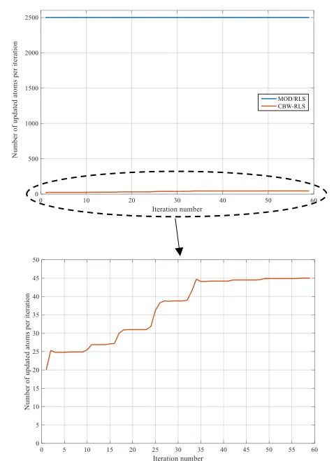
In order to compare the proposed method with the existing methods, the number of updated atoms as well as used data in each iteration of the algorithm and also percentage-root-mean square difference (PRD) are computed. Fig.1 shows the number of the updated atoms at each iteration for both MOD/RLS and CBW-RLS algorithms using the BCI Competition IV dataset. The comparison of the two graphs shows that in the proposed method, at the beginning, a small set of the atoms are updated (which equals to the sparsity level) and then with the addition of more data, this set becomes larger. Because of the low-rank property of multi-channel EEG signals (due to the correlation between different channels), non-zero elements of the sparse coefficient matrix are placed in the same rows, therefore, a few atoms contribute in the dictionary update stage. As Fig. 1 shows, after 59 iterations, just 45 atoms of the dictionary are updated, while in MOD/RLS, at every iteration all of the 2500 atoms participate in the dictionary update stage.
Figure 2 represents the number of data used at each iteration of CBW-RLS and a sample batch algorithm that is MOD, using the BCI Competition IV dataset. Batch methods such as MOD use the whole dataset to update the dictionary, while in the proposed method, at each iteration, only those EEG data which are correlated with the new one are used in the dictionary update stage. The red graph shows the number of data used at each iteration in CBW-RLS. Increasing the iteration causes a linear increase in the number of needed data. It is obviously seen that
Fig. 1 Number of updated atoms per each iteration in both MOD/RLS and CBW-RLS algorithms. This chart is averaged over 10 trials (m=2000, n=2500, L=59, SNR=20,
at each iteration, CBW-RLS uses much fewer training data to update the dictionary compared to the batch methods such as MOD.
Fig. 2 The number of data used per each iteration in both MOD and
CBW-RLS algorithms. This plot is averaged over 10 trials (m=2000, n=2500, L=59, SNR=20)
In order to evaluate the quality of the signal reconstruction, we compared the proposed method with RLS (1), RLS (10), ODL, GAW-RLS (1) and GAW-RLS (10). The term (1) means that the algorithm is executed just for one time over the whole dataset, while (10) means that it is executed for 10 times (The obtained dictionary at the end of the first cycle is used as an initial value for the second one and so on). Compression ratio is used to represent the amount reduction in the size of data representation and is expressed as:
Uncompressed size m CR=
Compressed size = k (27) where m and k are the dimensions of the original and compressed signals, respectively.
One commonly used criterion for assessing the quality of the signal reconstruction is PRD; that is the amount of distortion between the matrix of the original EEG signals Y and the matrix of the reconstructed signals , which is defined as:
2
F 2 Y F Y Y PRD=100
Y-μ
(28)
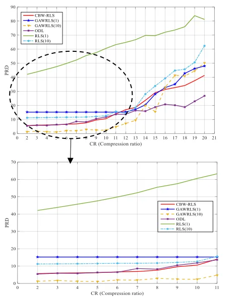
where μYis a vector containing the column-wise mean of the original matrix, Y. To compare the quality of the signal reconstruction, we used both of the aforementioned datasets and their results are plotted in figures 3 and 4, which show the PRD versus CR for BCI Competition IV and seizure datasets, respectively.
Fig. 3 PRD versus CR for BCI competition IV dataset
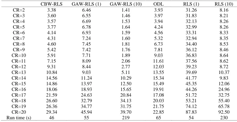
In order to more extensively compare the compression performance of the proposed CBW-RLS algorithm to the existing methods including GAWRLS, ODL and RLS, the PRD versus CR are given in Tables 1 and 2, for the two datasets of BCI Competition IV and seizure, respectively.
By investigating Tables 1 and 2, it can be observed that at low compression ratios, GAW-RLS (10) outperforms the other algorithms in term of reconstruction quality although at the cost of higher runtime. At high compression ratios, the proposed method CBW-RLS and ODL, both have the best performance in reconstructing compared to the others (the runtime of the proposed method is the lowest).
CBW-RLS GAW-RLS (1) GAW-RLS (10) ODL RLS (1) RLS (10)
CR=2 3.38 6.46 1.41 3.93 31.26 8.16
CR=3 3.60 6.55 1.46 3.97 31.83 8.21
CR=4 3.57 6.69 1.53 3.94 32.13 8.26
CR=5 3.77 6.78 1.64 4.24 32.99 8.26
CR=6 4.14 6.93 1.59 4.56 33.31 8.33
CR=7 4.31 7.24 1.60 5.32 32.94 8.35
CR=8 4.60 7.45 1.81 6.73 34.40 8.53
CR=9 5.42 7.42 1.76 7.81 36.12 8.46
CR=10 5.91 7.71 1.89 9.03 36.83 8.64
CR=11 7.15 8.09 2.06 11.61 37.56 8.62
CR=12 9.31 8.44 2.77 12.03 39.23 8.72
CR=13 10.84 9.03 5.11 13.55 39.69 10.37
CR=14 14.56 11.24 10.29 15.34 41.77 9.83
CR=15 14.86 13.97 12.50 15.49 45.35 12.06
CR=16 18.06 18.93 15.65 19.91 44.26 24.96
CR=17 21.59 24.63 20.84 17.08 51.72 32.75
CR=18 26.60 32.79 34.13 20.03 53.21 55.40
CR=19 26.36 34.77 31.75 21.75 74.12 65.78
CR=20 29.34 45.94 39.70 22.85 87.83 92.50
Run time (s) 46 55 219 65 54 230
CBW-RLS GAW-RLS (1) GAW-RLS (10) ODL RLS (1) RLS (10)
CR=2 5.64 15.22 1.24 5.42 42.10 11.22
CR=3 5.99 15.22 1.68 5.86 43.84 11.29
CR=4 6.08 15.22 1.20 5.74 45.71 11.35
CR=5 6.16 15.22 1.06 6.33 47.59 11.46
CR=6 6.67 15.22 2.00 6.45 49.85 11.59
CR=7 6.86 15.22 1.90 8.57 52.30 11.62
CR=8 7.60 15.22 2.88 8.22 55.48 11.74
CR=9 9.60 15.22 2.46 10.45 57.50 12.10
CR=10 10.56 15.22 2.40 11.84 60.56 12.68
CR=11 13.99 15.23 4.75 13.65 63.23 15.61
CR=12 16.92 15.35 7.12 13.65 64.84 14.33
CR=13 18.57 17.13 9.42 16.39 66.72 18.54
CR=14 23.61 20.41 20.03 15.89 69.80 28.06
CR=15 29.07 28.05 15.55 18.80 69.62 33.80
CR=16 31.33 32.64 32.81 20.79 72.05 39.22
CR=17 32.69 35.11 41.40 20.14 73.63 44.80
CR=18 34.15 42.79 40.97 18.76 75.98 45.69
CR=19 37.60 46.17 44.57 22.89 83.86 50.70
CR=20 41.36 48.05 50.19 26.76 81.17 62.40
Run time (s) 19 27 78 27 20 108
Table 1 PRD versus CR for BCI Competition IV dataset (The runtime of each algorithm is given as the last row)
6. Conclusion
In this paper, we introduced a new recursive least squares approach in dictionary learning problem to efficiently sparsify data to be used in compressed sensing scheme. In order to design the dictionary, between-channel correlations of EEG signals are exploited, leading to fewer number of data participate in the dictionary update procedure, which increases the speed of the algorithm, while reducing the computational complexity. After sparsifying the EEG signals using the proposed method, the sparse binary matrix is used to compress the EEG signals and in the reconstruction stage, OMP algorithm is applied. By assessing the simulations results of applying the proposed method on BCI Competition IV and seizure datasets, it can be concluded that the proposed method has better performance in terms of both the quality of the reconstruction and the speed of the algorithm compared to the other algorithms.
References
[1] Sanei, S.: Adaptive processing of brain signals. Wiley, Hoboken (2013) [2] Eldar, Y.C., Kutyniok, G.: Compressed sensing: theory and applications.
Cambridge University Press, Cambridge (2012)
[3] Mairal, J., Bach, F., Ponce, J.: Task-driven dictionary learning. IEEE Trans. Pattern Anal. Mach. Intell. 34(4), 791-804 (2012)
[4] Elad, M., Aharon, M.: Image denoising via sparse and redundant representations over learned dictionaries. IEEE Trans. Image Process. 15(12), 3736-3745 (2006)
[5] Xu, Y., Bao, G., Xu, X., Ye, Z.: Single-channel speech separation using sequential discriminative dictionary learning. Signal Process. 106, 134-140 (2015)
[6] Mairal, J., et al.: Supervised dictionary learning. Advances in Neural Inf. Process. Systems, 1033-1040 (2009)
[7] Zhan, X., Zhang, R., Yin, D.: SAR image compression using multiscale dictionary learning and sparse representation. IEEE Geoscience and Remote Sens. Letters 10(5), 1090-1094 (2013)
[8] Mallat, S.: A Wavelet Tour of Signal Processing. Academic Press, Cambridge (1999)
[9] Aharon, M., Elad, M., Bruckstein, A.: k-svd: An algorithm for designing overcomplete dictionaries for sparse representation. IEEE Trans. Signal Process. 54(11), 4311-4322 (2006)
[10] Fischer, S., Cristóbal, G., Redondo, R.: Sparse overcomplete gabor wavelet representation based on local competitions. IEEE Trans. Image Process. 15(2), 265-272 (2006)
[11] Donoho, D.L., Duncan, M. R.: Digital curvelet transform: Strategy, implementation, and experiments. Proc. SPIE 4056, (2000). https://doi.org/10.1117/12.381679
[12] Mairal, J., Bachm, F., Ponce, J., G. Sapiro, G.: Online dictionary learning for sparse coding. ICML '09 Proceedings of the 26th Annual International Conference on Machine Learning. (2009). https://doi.org/10.1145/1553374.1553463
[13] Smith, L., Elad, M.: Improving dictionary learning: Multiple dictionary updates and coefficient reuse. IEEE Signal Process. Lett. 20(1), 79-82 (2013)
[14] Sadeghi, M., Babaie-Zadeh, M., Jutten, C.: Learning overcomplete dictionaries based on atom-by-atom updating. IEEE Trans. Signal Process. 62(4), 883-891 (2014)
[15] Sadeghi, M., Babaie-Zadeh, M., Jutten, C.: Dictionary learning for sparse representation: A novel approach. IEEE Signal Process. Lett. 20(12), 1195-1198 (2013)
[16] Rubinstein, R., Bruckstein, A. M., Elad, M.: Dictionaries for sparse representation modeling. Proc. IEEE, 98(6), 1045-1057 (2010) [17] Pati, Y. C., Rezaiifar, R., Krishnaprasad, P.: Orthogonal matching pursuit:
Recursive function approximation with applications to wavelet decomposition. Proceedings of 27th Asilomar Conference on Signals,
Systems and Computers (1993). https://doi.org/10.1109/ACSSC.1993.342465
[18] Mallat, S. G., Zhang, Z.: Matching pursuits with time-frequency dictionaries. IEEE Trans. Signal Process. 41(12), 3397-3415 (1993) [19] Engan, K., Aase, S. O., Husoy, J. H.: Method of optimal directions for
frame design. Proc. IEEE International Conference on Acoustics, Speech, and Signal Processing. Proceedings (1999). https://doi.org/10.1109/ICASSP.1999.760624
[20] Skretting, K., Engan, K.: Recursive least squares dictionary learning algorithm. IEEE Trans. Signal Process. 58(4), 2121-2130 (2010) [21] Aviyente, S.: Compressed sensing framework for EEG compression.
Statistical IEEE/SP 14th Workshop on Statistical Signal Processing (2007). https://doi.org/10.1109/SSP.2007.4301243
[22] Lei, L., et al.: Multichannel EEG compression based on ICA and SPIHT. Biomedical Signal Processing and Control (20), 45-51 (2015)
[23] Ankita, S., Angshul Majumdar, A.: Row-sparse blind compressed sensing for reconstructing multi-channel EEG signals. Biomedical Signal Processing and Control (18), 174-178 (2015)
[24] Yipeng, L., De Vos, M., Van Huffel, S.: Compressed sensing of multichannel EEG signals: the simultaneous cosparsity and low-rank optimization. IEEE Transactions on Biomedical Engineering 62(8), 2055-2061 (2015)
[25] Hesham, M., Ward, R.: Block sparse compressed sensing of electroencephalogram (EEG) signals by exploiting linear and non-linear dependencies. Sensors 16(2), (2016)
[26] Naderahmadian, Y., Tinati, M. A., Beheshti, S.: Generalized adaptive weighted recursive least squares dictionary learning, Signal Process. 118, 89-96 (2016)
[27] Naderahmadian, Y., Beheshti, S., Tinati, M. A.: Correlation based online dictionary learning algorithm. IEEE Transactions on signal processing 64(3), 592-602 (2016)
[28] Blankertz, B., Dornhege, G.; Krauledat, M., Mller, K., Curio, G.: The non-invasive berlin brain-computer interface: Fast acquisition of effective performance in untrained subjects. NeuroImage 37(2), 539–550 (2007) [29] Goldberger, A.L., Amaral, L.A.N., Glass, L., Hausdorff, J.M., Ivanov,