http://www.sciencepublishinggroup.com/j/mlr doi: 10.11648/j.mlr.20190401.13
ISSN: 2637-5672 (Print); ISSN: 2637-5680 (Online)
Systematic Approach Towards Computer Aided Non-Linear
Control System Analysis Using Describing Function Models
Aparna Sadanand Telang
1, *, Prashant Prabhakar Bedekar
21
Department of Electrical Engineering, Faculty of P. R. Patil College of Engineering Management, Sant Gadgebaba Amravati University, Amravati, India
2Department of Electrical Engineering, Faculty of Government College of Engineering, Gondwana University, Chandrapur, India
Email address:
*Corresponding author
To cite this article:
Aparna Sadanand Telang, Prashant Prabhakar Bedekar. Systematic Approach Towards Computer Aided Non-Linear Control System Analysis Using Describing Function Models. Machine Learning Research. Vol. 4, No. 1, 2019, pp. 13-20. doi: 10.11648/j.mlr.20190401.13
Received: March 22, 2019; Accepted: April 30, 2019; Published: June 18, 2019
Abstract:
In recent years, control system problems involving non linearities are important concerns in the framework of automation industries. Actuators with non-linear behavior such as saturation, dead zone, relay, backlash etc. may be responsible for poor control performance in the system. The analysis of these non-linearities is an important task for a control system engineer. Moreover the methods of analyzing these non-linearities are time consuming and non-generic. This paper presents simple and systematic approach for analyzing such kind of non-linearities using user-friendly MATLAB tool “Nonlintool”. This tool saves the time as well as provides visual effects for analysis. Main contribution of this paper is to show how user friendly MATLAB tool “Nonlintool” can extensively be used for quicker and wider interpretation of results based on describing function models. The novelty of this paper lies in analyzing all kinds of non-linearities along with their impact on stability of the nonlinear system. The performance has been evaluated for varying conditions of magnitude and gain of the system as well as on various transfer function models. The results of stability analysis, for which only standard transfer function model is considered, are presented here.Keywords:
Nonlinear System, Non-Linearities, Transfer Function, Describing Function (DF), Nonlintool1. Introduction
Every real control system is non linear and nonlinear system analysis is an important issue in modern control system engineering. No universal analytical technique exists that can cater to the demand of analysis of the effects of uncertainties and/ or non-linearities [1, 2]. Non linearities such as saturation, dead zone, relay, backlash etc. may be responsible for poor control performance if their presence in the control system design is not properly addressed [3]. Moreover, the methods of analyzing these non-linearities are time consuming and non-generic. The computer aided tool offers user friendly computational platform to analysis and design of nonlinear control system [4-7]. Role of these tools is to serve information about stability analysis and behavior of nonlinear systems. Various graphical methods like Describing function, Phase plane trajectory and Zome’s circle criteria are
theory in control systems. Describing functions analyses the influence of inherent and indispensable components of all mechatronic systems as well as mechanical subsystems [12]. The hard nonlinearities are the part of both mechanical subsystems (friction, backlash, hysteresis) and the control system (saturation, hysteresis). These nonlinearities can cause both desirable and undesired phenomena where their most significant manifestation is the existence of limit cycles. How to obtain a describing function for a non-linear system containing one such non-linear element and further analysis of limit cycles based on the representation of the non-linear element by describing function has been studied.
Nonlinear behavior is common in aerospace systems, where many kinds of nonlinearities can produce limit cycles or other phenomena that can affect the system overall behavior. Limit cycles play an important role in nonlinear systems, provided that many control loops with common nonlinearities like relay, hysteresis, and saturation can present them. Thus, a proper description of this nonlinear phenomenon is highly desirable. A strategy for the linearized analysis is the describing function method, which is a frequency domain approach that allows the limit cycle prediction and stability analysis. Authors propose a systematic way of multiple limit cycle determination, as well as the stability analysis of each one [13]. A novel analysis and design tool for nonlinear control system is presented [14]. The tool would greatly facilitate the simulation of nonlinear systems. The tool is expected to be useful in designing of nonlinear control systems along with the behavior study of nonlinear elements. The tool uses new generation of GUIs developed in MATLAB, which greatly enhance the user’s ease of operation. NelinSys-a custom toolbox for nonlinear control systems is an efficient tool for analyzing the nonlinearities in the control system engineering. Some study reveal the applications of this tool in order to solve certain tasks from nonlinear control theory along with its implementation in MATLAB/Simulink [15]. Overall the field of nonlinear control systems has a bright future since there are many important and interesting challenges. The applications of nonlinear control systems, such as energy, health care, robots, biology, and big data research, will make the advanced theories and technologies be developed quickly [16].
This paper presents an application of user-friendly MATLAB tool “Nonlintool” using describing function models. Behavior of various non linearities under varying gain and magnitude as well as their impact on stability has been analyzed. Results have been evaluated and presented here for the standard non linearities and the standard transfer function model.
2. Common Nonlinearities and Analysis
of Nonlinear Systems
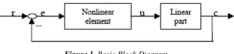
The non-linear systems where the principle of superposition no longer holds, is mainly composed of two parts viz. linear part and nonlinear part as depicted in Figure 1.
Figure 1. Basic Block Diagram.
Nonlinear part includes saturation, dead zone, ideal relay, friction, backlash, quantizer etc. Some of these non-linearities produce adverse effect on the system behavior and some have intentially to be introduced in the system for better performance of the system. Hence it is necessary to employ special analytical, graphical and numerical techniques which take account of these system nonlinearities. Commonly used methods of analysis of nonlinear systems are simulation method, perturbation method, phase plane and describing function methods.
Describing Function Method
A logical way to integrate a non-linear element into a linear control design problem is to describe this non-linear part by a describing function [6]. A describing function is always an approximation of the real situation. Describing function method is also called harmonic linearization method. This method is an approximate method to analyze nonlinear system and its main use is in stability analysis. It is also being the most practically useful method. Though it is an approximate method, it shows adequate accuracy in predicting whether limit cycle oscillations will exist or not in case of stability studies.
The describing function method provides a “linear approximation” to the nonlinear element based on the assumption that the input to the nonlinear element is a sinusoid of known, constant amplitude. The fundamental harmonic of the element’s output is compared with the input sinusoid to determine the steady state amplitude and phase relation. This relation is the describing function for the nonlinear element. It is represented by the function N(X), with X as input amplitude.
∅ (1)
Where X=Amplitude of the sinusoidal input signal. Y1=Amplitude of fundamental component of the output Φ1= the phase shift
3. Results and Discussions
The learning of nonlinear control system is somewhat difficult, complex and time consuming. MATLAB based GUI tool -‘nonlintool’ is easy and effective for studying the nonlinear control system based on proven graphical methods like DF, PPT, and Zames’ circle criteria. The tool is very generalized by providing facility for almost all types of nonlinearities and can explore various aspects of nonlinear control system very easily and effectively.
3.1. Analysis of Nonlinearities Using Describing Function Method
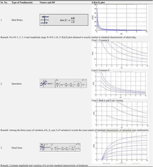
investigated by the method of Describing function. Table 1 illustrates the changes in describing function against different amplitude values of input of known discrete type of nonlinearities like ideal relay, saturation, dead-zone, amplifier with variable gain, relay with dead-zone, relay with hysteresis, backlash, hysteresis, friction, quantizer etc. One can know the behavior of selected nonlinearity by observing X /Kn(X) plot generated by this tool. The plot enables to understand how DF changes its value with increasing input value. Here different
parameter values of selected nonlinearity (like dead zone, saturation level, hysteresis value etc.) have been chosen and the behavior of the nonlinearity has been evaluated. From graph, the changes in the describing function against the different amplitude range of input X for various parameters have been easily understood. It is found that all nonlinearities whose input-output characteristics are represented by a planer graph, results into the describing functions independent of frequency but amplitude dependent.
Table 1. Changes in describing function against different amplitude values of input of known discrete type of nonlinearities.
Sr. No. Type of Nonlinearity Nature and DF X/Kn(X) plot
1. Ideal Relay
Remark: For M=1, 2, 3, 4 and Amplitude range X=0:0.1:10, X /Kn(X) plot obtained is exactly similar to standard characteristic of ideal relay.
2. Saturation
Case1: Constant k
Case2: Constant S
Case3: Both k and S are varying
Remark: Among the three cases of variation of k, S, case 2 of variation k reveals the exact nature of standard characteristic of saturation type nonlinearity.
3. Dead Zone
Sr. No. Type of Nonlinearity Nature and DF X/Kn(X) plot
4. Saturation with variable gain
Remark: Saturation with variable gain reveals standard characteristic similar to the characteristics of dead zone.
5. Relay with dead zone
Remark: Variation of M and constant amplitude implies approximate standard characteristics for this kind of nonlinearity.
6. Relay with hysteresis
1. Variation of M only
2. Variation of H and M both Remark: Changing M reveals constant phase angle plot.
7. Relay with dead zone and hysteresis
Remark: Changing M and H does not change the phase angle. This implies the describing function of the nonlinearity is independent of frequency.
Sr. No. Type of Nonlinearity Nature and DF X/Kn(X) plot
Remark: Larger backlash (gap b) leads larger phase lag which change the stability (in the form of limit cycle) and performance (poor).
9. Friction
1. Change of V0
2. Change of FC
3. Change of both Vo and Fc
Remark: Change of slope gain V0 with fixed amplitude FC reflects towards the constant amplitude X whereas Change of FC with fixed V0 reflects toward more linear characteristics.
10. Quantizer
3.2. Stability Analysis Using Method of Describing Function
Describing function techniques are also used to investigate the limit cycle behavior of the non-linear system. The method is best suited for the discontinuous non-linearities in control systems. A reliable prediction concerning limit cycle behavior can be obtained from this method. The limit cycle is predicted to be stable or unstable depending on the direction of crossing with respect to the linear system function in the Nyquist diagram. Stability analysis of system using DF is possible by using second module of the ‘nonlintool’. Here existence of limit cycle is being investigated on the basis of intersection of polar plot of linear part and plot of −1 /Kn(X). Stability of limit cycle is checked on the basis of direction of both the plots.
To predict the limit cycles and their stability, the non-linear part of the system is modeled as a describing function. Figure 1 depicts both linear block and nonlinear block. Different
kinds of transfer function models have been considered for linear block and various nonlinearities for nonlinear block. But to avoid lengthiness of the research work standard transfer function, as depicted below, as well as few standard nonlinearities have been considered here for stability analysis.
Context to the Figure 1, linear block of the transfer function is considered as-
G(s) = (2)
And nonlinearities chosen for nonlinear block as-
3.2.1. Ideal Relay
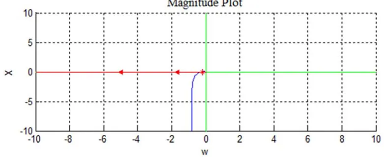
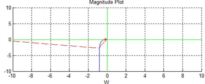
Stability analysis results of nonlinear system given in Figure 2. It shows that for given system, limit cycle exist with frequency about 2.44949 rad/sec and amplitude 0.5093. It also finds that the limit cycle is stable.
Figure 2. Stability of system with Ideal Relay.
3.2.2. Dead Zone
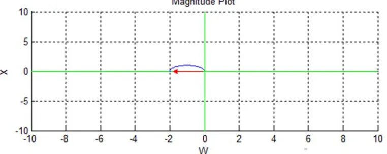
Stability analysis results of nonlinear system given in Figure 3. It shows that for given system, limit cycle exist with frequency about 2.44949 rad/sec and amplitude -0.491465. It also finds that the limit cycle is unstable.
Figure 3. Stability of system with Dead zone.
3.2.3 Relay with Dead Zone
Figure 4. Stability of system for relay with dead zone.
3.2.4. Relay with Hysteresis
Stability analysis results of nonlinear system given in Figure 5. It shows that for given system, limit cycle exist with frequency about 2.44949 rad/sec and amplitude 0.2546. It also finds that the limit cycle is stable.
Figure 5. Stability of system for relay with hysteresis.
3.2.5. Relay Dead Zone with Hysteresis and Dead Zone
Stability analysis results of nonlinear system given in Figure 6. It shows that for given system, limit cycle exist with frequency about 2.44949 rad/sec and amplitude 0.2. It also finds that the limit cycle is unstable.
Figure 6. Stability of system for relay with hysteresis and deadzone.
3.2.6. Backlash
Figure 7. Stability of system for relay with hysteresis and deadzone.
4. Conclusion
Applications of MATLAB GUI based tool ‘nonlintool’ for a nonlinear control system have been demonstrated in this paper. This tool provides good help for the analysis of nonlinear control system. All kinds of non-linearities along with their impact on stability of the nonlinear system have been successfully analyzed. The performance has been evaluated for varying conditions of magnitude and gain of the system as well as on various transfer function models. The changes in the describing function against the different amplitude range of input X for various parameters have been easily understood. The results for stability analysis using describing function method have been investigated for various nonlinearities as well as for transfer function models. Such kind of systematic approach towards the study of nonlinear systems proves to be one of the promising steps in the era of nonlinear control system engineering.
References
[1] A. Isidori, “Nonlinear control systems,” New York-Springer-Verlag, 1989.
[2] M Gopal, “Control Systems Principles and Design,” Tata McGraw- Hill, 2010.
[3] Giacomo Galuppini, Lalo Magni, Davide Martino Raimondo, “Model predictive control of systems with dead zone and saturation,” Control Engineering Practice, vol. 78, pp. 56–64, 2018.
[4] Anatoly Gaiduk, Nadežda Stojković, Elena Plaksienko, “Analytical Design of Nonlinear Control Systems,” Automatic Control and Robotics,” vol. 15, no 3, pp. 147-157, 2016. [5] R. R. Kadiyala, “A tool box for approximate linearization of
nonlinear systems in Control Systems,” IEEE on Control Systems, vol. 13, no. 2, pp. 47-57, April 1993.
[6] Xueling Song, Chaoying Liu, Zheying Song, Yingbao Zhao, “The Design of Software Platform for Nonlinear System Analysis,” International Conference on Computer Science and Software Engineering, pp. 875-878, 2008.
[7] R. M. R. Bruns, J. F. P. B. Diepstraten, X. G. P. Schuurbiers, J. A. G. Wouters, “Motion Control of Systems with Backlash,” Master Team Project, pp. 1-50, August 2006.
[8] P. Shab and J. B. Patel, “Learning of Nonlinear Control System Using nonlintool,” IEEE Fourth International Conference on Technology for education (T4 E), IIIT- Hyderabad, pp. 184-187, 2012.
[9] Sergey Ul'yanov, N. N. Maksimkin, “Software toolbox for analysis and design of nonlinear control systems and its application to multi-AUV path-following control,” 40th International Convention on Information and Communication Technology, Electronics and Microelectronics (MIPRO), pp, 1032-1037, May 2017.
[10] E. A. Freeman, “Dynamic analysis of nonlinear control systems,” PROC. IEE, vol. 114, no. 1, pp. 129-138, January 1967.
[11] Derek P. Atherton, “Early Developments in Nonlinear Control,” IEEE Control, pp. 34-43, June 1996.
[12] S. Dormido, F. Gordillo, S. Dormido-Canto, J. Aracil, “An Interactive Tool For Introductory Nonlinear Control Systems Education,” 15th Triennial World Congress, IFAC Elsevier publication, pp. 255-260, 2002.
[13] Zdeněk Úředníček “Nonlinear systems - describing functions analysis and usings,” MATEC Web of Conferences, pp. 1-10, 2018.
[14] Alexandro Garro Brito “Computation of multiple limit cycles in nonlinear control systems-a describing function approach,” J. Aerosp. Technol. Manag., vol.3, no.1, pp. 21-28, Apr. 2011. [15] Jaydeep Jesur, Ashay Shah and Jignesh B. Patel, “Nonlintools:
GUI Tool for Analysis and Design of Nonlinear Control System,” Nirma Universitty Journal of Engineering and Technology, vol.1, no.1, pp. 34-37, Jan-Jun 2010.
[16] M. Ondera “MATLAB-Based Tool for Non-Linear Systems,” CEEPUS Summer School Intelligent Control Systems, pp. 1-15, 2005.