Investigation of Clustering in Turing Patterns to describe the Spatial Relations of Slums

Investigation of Clustering in Turing Patterns to

describe the Spatial Relations of Slums

Jakob Hartig1, John Friesen1∗ ID _{and Peter F. Pelz}2ID

1 _{Chair of Fluid Systems, Technische Universität Darmstadt, Otto-Berndt Str. 2, 64289 Darmstadt, Germany}

* Correspondence: [email protected]; Tel.: +49-6151-16-27100

Abstract:Worldwide, about one in eight people live in a slum. Empirical studies based on satellite data have identified that the size distributions of this type of settlement are similar in different cities of the Global South. Based on this result, a model was developed that describes the formation of slums with a Turing mechanism, in which patterns are created by diffusion-driven instability and the inherent characteristic length of the system is independent of boundary conditions. It has not yet been taken into account that Turing patterns usually arrange themselves regularly, while slums are often found in clusters. Therefore, this study investigates to what extent a common reaction kinetics for Turing models can be adapted to represent a locally concentrated arrangement of objects and to adapt the size distribution of the objects to the empirical results. Based on a summary of the literature and two numerical studies, it can be shown that although it is possible to adapt the model to the empirical data, this also increases the complexity of the model.

Keywords:slums; informal settlements; bifurcations; Turing pattern

1. Introduction

The United Nations estimate that around 1 billion people worldwide live in slums [1]. In recent years, the number of analyses of these settlement types has been steadily increasing [2–4]. Often the studies are based on satellite data, since their use allows a globally comparability. Since satellite data can be used to determine only the physical morphology of these settlements, conclusions about the social group living in them can only be drawn indirectly [5]. Therefore, this settlements are called morphological slums. Morphological slums are characterized by a high settlement density and organic, complex settlement structures. The buildings themselves are small relative to the buildings in the formal settlements in their surroundings and are characterized by low height. Friesen et al. [6,7] analyse the size distribution of morphological slums and find that in contrast to cities within a country, slums in eight different cities in the Global South show a similar size distribution with a similar geometric mean. This leads to the conclusion that regardless of culture, country and continent, a typical slum size of 0.01 km2exists. This corresponds to an edge length of 100 m for a square area. The size of most slums is between 10−3km2and 10−1km2and thus shows no dependence on the total number of morphological slums within the city. This information can be used as typical scale in other scientific domains such as infrastructural planning [8] or epidemiological analyses [9,10].

This studies on the similar size of slums were recently taken up by Pelz et al. [11] who put forward the hypothesis that the development of slums could be described by a Turing model. This is due to the fact, that a characteristic quantity can be observed in both Turing patterns and slums. Another motivation for this hypothesis is the work of Theraulaz et al. [12], who show that Turing patterns are also formed by higher organisms.

Pelz et al. [11] propose the thesis that the formation of slums results from the interaction of two social groups with different characteristics. The interaction of both groups is described by two coupled reaction diffusion (RD) differential equations, each of which represents a social group. The schematic division of the population into two groups, differing mainly in their mobility, is based on their income.

The main thesis is that these different mobilities lead to an instability of the equations, resulting in patterns with a similar size.

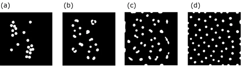
While the instability predicted by the model generates structures of the same size and distance, the sizes of the settlements in slums are similar, but the distances between them vary considerably (Figure1).

Figure 1.Qualitative visual comparison of slum patterns (a), [13] and simulated Turing patterns (b).

Comparing the pattern formation of slums 1a with the Turing patterns in Figure 1b, clear differences are already noticeable visually. Besides shape and size, the slums show an arrangement in which certain areas of the city are not covered with slums. In previous studies it was shown that slums are arranged in clusters [14]. Hartig et al. [15] confirms that and show a tendency towards random spatially distribution of slums within the clusters. Therefore, in this thesis we investigate the question whether it is possible to map the clustering we see in the empirical data with RD equations by varying the reaction kinetics spatially. Furthermore, it can be seen that the slums have a wider dispersion in the size distribution than the patterns in the RD equations. This aspect is also quantified and discussed in this paper.

To analyse these topics, the paper is structured in the following way: First, we shortly present the model of Pelz et al. [11] (sec. 2.1). Afterwards, we present methods from the literature, dealing with pattern formation in RD equations for inhomogeneous parameters (sec. 2.2). In a next step we perform two parameter studies in order to quantify the relationship between the variing parameters (reaction (sec. 3) and diffusion parameter (sec. 4)) and the resulting patterns. While the first investgates the possibility to impliment clustering in the RD model, the second investigates the width of the size distribution. We use the well-known approach of Schnakenberg, one of the simplest equations leading to Turing patterns [16]. We then discuss the results in each section and finally conclude (sec. 5) our paper.

2. Model and Methods

In this section, we shortly recapitulate the model of Pelz et al., present concepts from literature, were inhomogeneous parameters were investigated and show the ideas and methods, we pursue in this paper.

2.1. Model by Pelz et al.

∂ue1 ∂et

=UR fb ₁(u₁,u₂) +D₁∆eu₁, ∂ue2

∂et

=UR fb ₂(u₁,u₂) +D₂∆eu₂. (1)

e

uidescribes the density fields of both population groups (i=1 represent “rich”,i=2 represent “poor”),Ub the popultion density,D_ithe diffusion coefficients,Rhas the dimenson of a rate andf_iare

the coupled reaction rates.

They bring the equation into a dimensionless form by using the following parameterst:= Ret, xj :=exj

√

R/D1,ui :=uei/Ubyielding to

∂ui

∂t = fi(uj) +dij

∂2uj ∂xk∂xk

, dij= 1 0 0 d

!

(2)

withd:=D2/D1. As the study was presented by Pelz et al. on a conceptual level, the parameters

presented so far were sufficient. In this paper an additional dimensionless parameterγ=l2R/D1is

introduced. This quantity is the shape parameterγand is necessary if calculations or simulations are performed on a limited area of lengthl.

∂ui

∂t =γfi(uj) +dij

∂2uj ∂xk∂xk

(3)

To identify the the conditions, where Turing pattern occur, a linear stability analysis with the following approachδuj=R[δubjexp(σt+ikkxk)]is conducted, leading to the following eigenvalue problem:

(σδij−bij)δu_bj=0,bij:=γaij−k2dij (4) with the Jacobianaij:=∂fi/∂uj, the Kronecker deltaδij, the eigenvalueσand the Euclidian length k=√kikiof the wave vectorki. A solution to the eigenvalue problem exists, if

det(σδij−bij) =0 (5)

This results in the following dispersion relation:

σ1,2 = 1

2bii± q

b2_ii−4 det(bij) (6) For a state stable in the absence of diffusion to become unstable, the following two conditions must be met: (i)R(σ)<0, ifdij=0 and (ii) for at least onek6=0 the real part ofσhas to be positiveR(σ)>0. This is given under the following conditions, wheretris the trace of the matrixbij:

−tr(bij)>0 (7)

detbij>0 (8)

(da11+a22)2

4d >det(aij) (10)

If these conditions are fulfilled, which can be achieved as shown here by an increasing value of the diffusion coefficient. If one understands the different diffusion coefficients as different mobilities of the two social groups to move within the city, this characteristic can be understood as a cause for the formation of slums.

2.2. Literature review on pattern formation with inhomogenous parameters

With homogeneous parameters in the Turing space, if the reaction area is sufficiently large for the unstable wavelengths, Turing patterns are formed in the entire reaction area with homogeneous wavelengths. This means in particular that after convergence the whole area is covered by patterns. Which of the possible unstable wavelengths emerges is determined by mode selection [17]. The assumption of locally homogeneous parameters is naturally not always correct in real systems. Especially Maini deals with the question of the effects of inhomogeneous parameters on Turing patterns. In systems with parameter fluctuations, the height, width and distance of concentration peaks can be influenced. Page, Maini and Monk [18] show both by a disturbance calculation, as well as numerically on a Gierer-Meinhardt system, that a local parameter variation leads to complex pattern formation. For very smalld=D2/D1applies,

• expansion of the acitvator peaks∝√D1

• distance between the acitvator peaks∝√D2

• height of the activator peaks∝√D2/D1

Variing the parameters with a wavelength, the wavelength has an influence on the emerging wavelengths of the system. If the wavelengths of variation are much larger than the natural wavelength of the RD system, then the resulting pattern has the natural wavelength with an amplitude modulation in the amount of the parameter variation. If the wavelength of the fluctuations is smaller than the wavelength of the RD system, then only harmonics of the parameter variation appear [18].

2.3. Framework and reaction kinetics

As discussed in the literature review, there are different ways to change the pattern formation in RD systems. With regard to our application we investigate two different questions:

1. Can the cluster formation observed in slum systems be implied by spatial variation of the reaction kinetics in RD equations?

2. Can the width of the size distribution be changed by spatial variation of the diffusion coefficients?

To answer these questions, we first have to introduce reaction kinetics. There are many different reaction kinetics known in the literature (cf. [23]), probably the simplest is the one of Schnakenberg [16]. The two coupled reaction terms have the following form:

f1(u1,u2) =a−u1+u21u2

f2(u1,u2) =b−u21u2. (11)

These reaction kinetics will be integrated in eq. 2 and the resulting system is analysed in the follwing sections.

3. Analysis of spatial varying reaction coefficients

Turing patterns result from instability. Since every point in an area is unstable, when the inital conditions are homogenous, there is no preference for certain space points at the beginning. Initial condition does not ensure a spatially limited arrangement of concentration peaks when the patterns converge, because, for example, there is no attractive field between concentration peaks. This can impressivly be shown in Figure 2, where starting from clustered inital conditions and spatially homgeneous parameters, the pattern merge into a homogeneously arranged pattern.

Figure 2. Qualitative illustration of a Schnakenberg system with clusters as initial condition and homogeneous parameters. Initial condition (a)t=0, (b)t=0.16t=tend, (c)t=t=0.27tendand end (d)t=tend.

To achieve this symmetry and to integrate the results of the data analysis into the model, could two methods can be identified by the literature search (see Sec. 2.1):

1. restriction of instability to a specific area by areas with parameters in Turing space and areas with parameters outside the Turing space.

2. local pattern formation outside the Turing space by jumping in the parameter.

For the second method, due to a lack of knowledge about the parameter range, with the local pattern formation occurs through a parameter jump, a parameter study required. In the parameter study, both methods can easily be tried out. Numerical simulations are used as a method. For simulation the program FlexPDE from PDE Solutions Inc. in version 6.50n/W64 is used. It is a Finite element program (FEM program) for the solution of partial, time-dependent Differential equations. Meshing takes place automatically and is performed during the solution process adapted. The fineness of the mesh can be determined by a budget of mesh nodes.

3.1. Parameter study

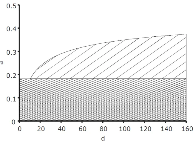
First of all, a parameter study is conducted to identify the region of parameters in which local limited Turing patterns occur due to parameter jumps. The kinetics parameterbis initially set arbitrarily tob=0.5. The Turing space then looks as shown in Figure3.

Figure 3. Turing space (hatched), area with unstable kinetics without diffusion (crosshatched) for Schnakenberg kinetics with fixed parameterb=0.5.

There will be a jump in the kinetics Parameteraexamined. The reaction area is divided into two subareas in which all parameters are equal, exepta(Fig.4a). The Turing space as well as the area above it is defined with of different numbers of points are covered.

With initial parameter studies, which are not documented here, the parameter range ofa,dand the step height are limited and it is ensured that the resulting patterns are largely converged out after the break-off time. In these studies it has been found that the crosshatched area in Figure3, where the kinetics are unstable, is not a useful parameter range for simulations. Patterns do not arise there. In the restricted parameter range, 100 simulations are performed, where the parametersaand dwere varied as shown in Figure4b. The simulation time for each simulation ist = 50, the size parameterγ=70, the boundary conditions are no-flux boundary conditions, the initial conditions are the stationary solution of the kinetics where the componentu1is randomly increased by 1 % by the

stationary solutionu1,0=a+bis varied. Since the componentsu1andu2are inverse, in the following

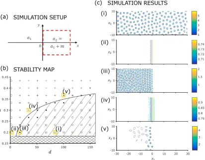
Figure 4.(a) Setup of the simulation area to investigate the influence of a jump of kinetic parametera bym. (b) Parameter study in the Turing Room with 100 points. The points are examined parameter sets. Shown is the kinetics parameter left of the jump,a1. The value to the right of the jump is always a2=a1+0.05, the parameterb=0.5. The results of the parameter study are coded as follows: Turing pattern in the whole area ( ), Turing pattern in the left half (•), no pattern (◦), localized stripes (+), localized points (*). (c) (i) Turing pattern on both sides of the jump (a1=0.2,d=80.5), (ii) no Turing pattern, just the concentraion difference due to the jump (a1=0.2,d=1), (iii) Turing pattern on the left side of the jump with parameters in the Turing space. No pattern on the right side of the jump, since parameter is outside of the Turing space (a1=0.2,d=18), (iv) stripe pattern, parameters outside of the Turing space (a1=0.3,d=34.5.5) and (v) Turing pattern left of the jump with parameters outside of the Turing space (a1 =0.3667,d=100.5). The edgy patterns on the left of (c,v) are the result of meshing, as the number of nodes is limited and the main part is used to map the jump.

In the results, five basically different solutions are observed, which are qualitatively different and can be distinguished by the resulting patterns and the position of the parameters in space:

1. dot pattern in the whole area. With this result the parameters are all in the Turing space. As expected, Turing patterns are created. Optically there is no difference in the distance and size of the points between the halves of the simulation space.

2. no patterns on either side. Here all parameters are outside the Turing space. As expected, no patterns are created.

3. dot pattern in one half.In this case the parameters left of the jump are inside the Turing space, the parameters right of the jump are outside. Therefore patterns are concentrated in one half of the simulation space.

5. dot patterns in one half, which become smaller with distance from the jump.The parameters are outside the Turing space here too. But there are dot-like patterns that disappear with distance from the jump.

In principle, the results found in the parameter study correspond to results from [20] and [22]. Two methods can be used to create spatially limited Turing patterns will be. On the one hand, by limiting the instability to one side locally restricted (case 3). On the other hand, excited by a parameter jump, local limited Turing-pattern occur outside of Turing space (here case 4 and 5). It can also be shown, that in the system with Schnakenberg kinetics in the chosen parameter range these patterns appear as points only in the surrounding of the Turing space. (see Figure4b). At a greater distance from the Turing space locally limited stripes are formed, which decrease in amplitude with distance. This behaviour shows parallels to the results from [19]. In this thesis a changed bifurcation structure is observed by non-constant parameters.

3.2. Influence of shape

The generic investigations of the previous section are a first step to illustrate cluster formation with RD equations. In a further step the influence of the shape of a jump is to be considered. For this purpose, a polygon is defined, with the jump running transverse to its edge.

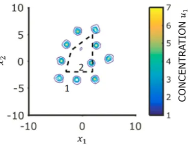
Figure 5. Simulation of a jump in a with a course transverse to polygon (dashed). Parameters: a1=0.4,a2=0.45,d=133.5,b=0.5,γ=70,t=100.

The pattern formation starts at about 10% of the total simulation time. The first Concentration peaks occur at the corners. In the course of time these migrate outwards and other spikes appear in between. As can be seen in Figure5, the but not all points outside the polygon. Altogether the concentration peaks in the shape of the polygon.

3.3. Discussion

With the parameter study it can be shown that, as described in the literature, local pattern formation by jump excitation also occurs outside the Turing space. This is possible, because due to the parameter jump the conditions for the derivation of the Turing space are no longer valid. Within the Turing space, as expected, pattern formation occurs in the whole area. A second form of local pattern formation also occurs in the results if the parameters on one side of the jump in the Turing space, but on the other hand outside.

of parametersbandγ, nor any other parameters thanaanddwith a larger parameter range have been investigated, but represent a possible solution in principle.

The patterns that are created by a jump in a kinetics parameter are induced, but do not tend to form natural clusters, but only to local pattern formation around the jump. There is no attraction between the concentration peaks, which leads to clustering. Clustering with regard to the total reaction area can therefore only be created by a prepattern in the form of a jump. The shape of the prepattern determines the quality of the model. To adapt the resulting patterns to real data, the results of previous analysises [15] can serve as a basis for a prepattern. They show that a characteristic cluster size for slums, which varies from city to city which is in the order of 103m. The cluster size can be set in the model to different ways to bring the model in line with reality bring.

A second method could be to use the characteristic cluster size to set up models only within clusters, that is, to limit the validity of the model to the cluster size. Both methods require prior knowledge in the form of pre-patterns or a validity range and therefore take away the simplicity of a few parameters from the model.

However, Turing has also described that the analytically manageable case of pattern formation from the homogeneous initial state can only be the exception and not the rule "Most of an organism, most of the time, is developing from one pattern to another, rather than from homogeneity into a pattern." [24] This statement is also valid for the city system, because geography, history of the city, culture and the surrounding area influence the respective picture of a city. A slum model must, to be plausible, certainly have some of these influences image. A prepattern is a way to do this without using the model of the RD equations to change things.

4. Analysis of spatial variation of diffusion coefficients

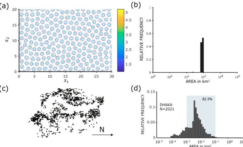
Figure 6.(a) Resulting pattern by homogeneous parameters (a=0.2,b=1,d=50,γ=70,t=50). (b) Size distribution of concentration peaks from (a) with a threshold of 2. (c) Empirical spatial pattern of the slums of Dhaka (2010) from [13].d) Size distribution of (c).

Page, Maini et al. show that especially locally varying parameters lead to a modulated wavelength in the patterns [18]. Therefore, in the following the influence of locally monotonically varying diffusion coefficients will be investigated. As described in section 2.2, there is a relationship between the wavelength and the resulting pattern size. Influencing the wavelength therefore also leads to a wider size distribution.

4.1. Parameter study

However, RD-Eq. 3 cannot be used to represent locally varying diffusion coefficients, but must be derived from the more general form. In general, the derivations for the Turing space are no longer valid. If one assumes a system which is undimensioned except for the diffusion coefficients, then the initial equation becomes

∂u1

∂t =∇ ·D1(x1,x2)∇u1+γ(a−u1+u

2 1u2)

∂u2

∂t =∇ ·D2(x1,x2)∇u2+γ(b−u

2

1u2). (12)

To de-size eq. 12, Di(x1) is split into a constant mean diffusion coefficient ˆDi and a location-dependent function gi(x1). The mean diffusion coefficients are then undimensioned in

the conventional way. This results in

∂u1

∂t =∇ ·g1(x1,x2)∇u1+γ(a−u1+u

2 1u2)

∂u2

∂t =d∇ ·g2(x1,x2)∇u2+γ(b−u

2

Eq. 13 is used as the basis for the simulations in this chapter, withgi(x1)being specified in more

detail. Jumps for mapping for size distributions with varying diffusion coefficients are not advisable, since many jumps would be necessary for a size distribution. This would involve very long calculation times and the model would not be numerically practicable. In the following, therefore, the influence of the wavelength of the Turing patterns by means of the local dependence of parameters on smooth functions is analysed.

4.2. Spatial variation of diffusion

In order to find the connection between the change in diffusion coefficients over the location as well as the size of the resulting patterns,gi(x1,x2)is first defined as a linear function. A rectangular

area is defined on the equation 13 with

gi(x1,x2):=1+mix1 (14)

depends on a direction in space. The slope parametermi is set equal to zero or as a positive number, depending on whether the diffusion coefficient ofu1oru2is to be varied. The parameters for

all investigations area=0.2,b=1,d=50,γ=70,t=50. The initial conditions are the homogeneous initial state, whereu1, 0 is randomly varied by 1 %. The threshold for the simulation is 10−4foru1and

u2, the error limit is 10−5, the number of nodes is limited to 10000.

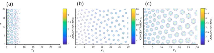
With the variation ofg1(cf. Figure7a), the patterns only occur in a part of the reaction area. The

concentration decreases with increasingx1until the patterns are not are more visible. The distance

between concentration peaks remains constant. At variation ofg2(cf. Figure7b), on the other hand,

the patterns emerge in the whole reaction area. The concentrationu1increases asx1increases. The

diameter of the Pattern seems to be slightly larger with increasingx1 , the distance between the

concentration peaks seems to remain constant.

Figure 7.(a) Spatial pattern forg1 =1+0.25x1andg2=1 (b) Spatial pattern withg2 =1+0.25x1 andg1=1. (c) Spatial pattern withg1=1+0.25x1andg2=1+0.25x1.

Varying bothg1andg2, the points become larger with x1(see Figure7c). The concentration

abovex1remains the same, the distance between concentration peaks increases. To determine the

development of the point size quantitatively, we conduct further investigations.

With a threshold of 2 the concentrationu1is converted into a binary pattern, meaning that all

points withu1>2 are set to 1, all points withu1<2 are set to 0. From this binary pattern we find the

sizes of the concentration peaks depending on the location. The points at the edge of the simulation area were excluded from the analysis using a suitable filter method so as not to falsify the result.

Figure 8.(a) Display of the dependence of the area on the position inx1direction in the simulation area for different with variation ofg1andg2.The area is undimensioned over the total area of the grid. (b) Nearest-Neighbour-Distance plotted over the position. (Similar to (a))

Especially the results from of the simulation withm=0.25 are additionally divided into smaller groups. The latter can be explained by the fact that the points in the patterns are more or less parallel to thex2-axis. Points of a size are thus located approximately at a position in x1-direction. The

arrangement in a line indicates a dependence of the formA ∝ √x1. To verify this, the empirical

correlation coefficient betweenAand√x1each of the simulations is determined. The results for this,

as well as the results of a linear regression, are summarized in Table 1. Since the correlation coefficients in all three cases are very close to 1, a linear relationship can be assumed in Figure8a andA∝√x1is

thus confirmed.

Table 1.Results from the regression of the data from Fig. 5a.

Simulation Correlationcoefficient Slope Intercept

m=0.25 0.9816 0.1073 -0.0203

m=0.5 0.9792 0.2063 -0.1413

m=0.75 0.9876 0.2966 -0.2140

The change in the distance is measured using the Nearest-Neighbour-Distance, i.e. the Distance of each point to its nearest neighbour, quantitatively evaluated, since an optical assessment based on the simulation results is difficult. For the simulations in whichg1andg2are varied at the same

time, Figure8b. The course of the points is similar to the course of the points in Figure8a. the points from each of the three cases arrange themselves on a line, with each line divided into smaller groups. Also for the other cases, where either onlyg1or onlyg2are varied, the result is a similar course (not

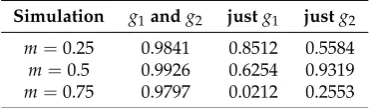
shown). The correlation coefficients give a similar picture as in the analysis of the areas. The connection between the Nearest-Neighbour-Distance and√x1is the for the variation ofg1andg2linear. For the

other cases, where either onlyg1or onlyg2is varied, no linear relationship is apparent. Since both the

area and the Nearest-Neighbour-Distance are equally affected by√x1this implies a proportionality

Table 2.Correlation coefficients for nearest neighbour distance and area

Simulation g1andg2 justg1 justg2

m=0.25 0.9841 0.8512 0.5584

m=0.5 0.9926 0.6254 0.9319

m=0.75 0.9797 0.0212 0.2553

4.3. Discussion

In summary, it can be said that a linear change in the diffusion coefficients over a separation has various effects on the height, distance and area of the concentration peaks that are produced. Thus, the mode selection of Turing patterns can be negated by inhomogeneous diffusion coefficients. The effects of the variation of individual diffusion coefficients are summarized in Table 3 for better clarity.

Table 3.Summary of the qualitative influence of linear location dependence on pattern formation.

Variation of heigth of peaks distance area

g1andg2 constant increases increases

justg1 decreases constant decreases

justg2 increases increases increases

The height of the concentration peaks decreases with increasingf1and increases with f2. These

effects cancel each other out for simultaneous variation ofg1andg2. The area decreases withg1and

increases withg2. If one compares these results qualitatively with the results from [18], the results are

confirmed only for the height of the peaks. The results for the area and distance cannot be confirmed. In principle, the distance in the simulations of this work shows the same dependencies as the surface. Distance and area are therefore proportional to each other. This common increase shows that pattern formation by RD equations is a strongly coupled phenomenon. The difference between the results found here and the work may be due to the fact that a Schnakenberg kinetics is investigated here, while the authors of [18] investigate a Gierer-Meinhardt kinetics. Furthermore, the authors use an interference approach for which the ratio of the diffusion coefficientsdmust be much smaller than 1. Here, however, the ratio isd=50. Furthermore, it can be shown that the area of the points and their distance increases proportionally with simultaneous and equal linear spatial dependence ofg1andg2.

Consequently, the square of the area is proportional to z or | when both diffusion coefficients are varied. With this insight, theoretically any size distribution can be constructed. However, this is a difficult and time-consuming problem compared to the reverse problem, the determination of a size distribution. An analogous problem can be found with drag coefficients of wing profiles. The determination of the coefficient of drag of a given wing profile is easily done by analytical or numerical calculations. Conversely, however, calculating an airfoil with a desired drag coefficient is difficult due to the large number of possible solutions. Therefore we will end at this point with the result that in principle a solution exists. More important is the question of the usability of this solution for the representation of slums by means of Turing patterns. With regard to this, the found proportionality of area and distance with variation of both diffusion coefficients is a problem, since no such strong correlation is observed in real slum data. The applicability of the approach investigated here is therefore questionable.

5. Conclusion

For these reasons Pelz et al. [11] stated the hypothesis that slums as anthropogenic patterns can also be mapped by Turing patterns. This model would have the advantage of a small number of parameters and sizes compared to common slum models (see [25]).

The clustering observed in the slum data sets cannot be found in Turing patterns. Rather, Turing patterns result in a homogeneous distribution of points in space. Moreover, unlike in slums, the size distribution of the points is narrow and dominates by a particular size. The reason is the mode selection in Turing patterns. Results from the literature suggest that the spatial arrangement and size of the pattern using non-homogeneous parameters. This is done using simulations have shown that jumps in one parameter of the reaction kinetics form spatially limited patterns. Parameter studies show that these local pattern formation takes place outside the Turing space. Cluster formation could be represented by a prepattern in form of jumps. To identify structures for the prepattern, the characteristic cluster size found in this work could be can be used. By means of locally equally dependent diffusion coefficients for both components in the RD equations, any size distribution of the resulting patterns can be achieved. However, this also changes the distance between the concentration peaks, which does not match the observed properties of the slums. The simulations show a proportionality between area and distance, whereas in slums diameter and distance are hardly related. Turing patterns have further properties which, unlike the resulting patterns, are not recognizable at first glance, but which must be found in the potential system to be mapped. These properties mainly concern the origin of the patterns and are therefore not directly visible in illustrations of the patterns. A comparison of the properties yields few matches. For example, when Turing-patterns are created, the concentration of both components changes simultaneously by interaction. In the case of slums, there is no simultaneous growth of slums and surrounding city, which is an indication against self-organization. Furthermore, in Turing patterns the wavelength of the patterns changes when the size of the area changes. This behavior is not observed in slums, since they have a characteristic size independent of the city under study.

This work shows show that there are differences between slum and Turing patterns, especially in the development of the patterns. However, without considering the process of formation, the slum patterns that emerge can basically be described with Create Turing patterns by considering heterogeneous parameters. With the However, the use of heterogeneous parameters, possibly coupled with a prepattern, is possible. the simplicity of the model through the interdependencies and more parameters as a great advantage.

The results of the work show that when mapping slums using Turing patterns there are already qualitative differences in the systems. The question therefore arises as to the reason for that. Apart from the answer that slums do not depict themselves with Turing patterns there could be other reasons. For example, one of the basic assumptions of this work could be to want to map the building structure, be wrong. Perhaps building structures or slums are a result of previous processes. Such approaches can also be found in the context of Turing patterns in biology. The Pattern formation by the Turing mechanism takes place in a much shorter time as the final expression of the patterns in the form of cell differentiation, for example [26]. Slums that do not grow simultaneously with the city surrounding them also need space, on which they can grow. So there must also be a previous pattern. Investigation of free surfaces and their properties could provide information about whether these surfaces can be described by Turing patterns. Slums then arise from this pattern and are in a sense a third component in the RD equations.

Author Contributions: Conceptualization, Jakob Hartig and John Friesen; Formal analysis, Jakob Hartig; Investigation, Jakob Hartig; Methodology, John Friesen; Project administration, Peter F. Pelz; Supervision, John Friesen and Peter F. Pelz; Visualization, Jakob Hartig and John Friesen; Writing – original draft, Jakob Hartig; Writing – review & editing, John Friesen.

Funding:This research received no external funding.

Conflicts of Interest:The authors declare no conflict of interest.

Abbreviations

The following abbreviations are used in this manuscript:

RD reaction diffusion

References

1. Ezeh, A.; Oyebode, O.; Satterthwaite, D.; Chen, Y.F.; Ndugwa, R.; Sartori, J.; Mberu, B.; Melendez-Torres, G.J.; Haregu, T.; Watson, S.I.; Caiaffa, W.; Capon, A.; Lilford, R.J. The history, geography, and sociology of slums and the health problems of people who live in slums. The Lancet2017,389, 547–558. doi:10.1016/S0140-6736(16)31650-6.

2. Kuffer, M.; Pfeffer, K.; Sliuzas, R. Slums from Space—15 Years of Slum Mapping Using Remote Sensing. Remote Sensing2016,8, 455. doi:10.3390/rs8060455.

3. Mahabir, R.; Crooks, A.; Croitoru, A.; Agouris, P. The study of slums as social and physical constructs: challenges and emerging research opportunities. Regional Studies, Regional Science 2016, 3, 399–419. doi:10.1080/21681376.2016.1229130.

4. Mahabir, R.; Croitoru, A.; Crooks, A.; Agouris, P.; Stefanidis, A. A Critical Review of High and Very High-Resolution Remote Sensing Approaches for Detecting and Mapping Slums: Trends, Challenges and Emerging Opportunities. Urban Science2018,2, 8. doi:10.3390/urbansci2010008.

5. Wurm, M.; Taubenböck, H. Detecting social groups from space – Assessment of remote sensing-based mapped morphological slums using income data. Remote Sensing Letters2018,9, 41–50. doi:10.1080/2150704X.2017.1384586.

6. Friesen, J.; Taubenböck, H.; Wurm, M.; Pelz, P.F. The similar size of slums. Habitat International2018, 73, 79–88. doi:10.1016/j.habitatint.2018.02.002.

7. Friesen, J.; Taubenböck, H.; Wurm, M.; Pelz, P.F. Size distributions of slums across the globe using different data and classification methods. European Journal of Remote Sensing 2019, pp. 1–13. doi:10.1080/22797254.2019.1579617.

8. Rausch, L.; Friesen, J.; Altherr, L.; Meck, M.; Pelz, P. A Holistic Concept to Design Optimal Water Supply Infrastructures for Informal Settlements Using Remote Sensing Data. Remote Sensing2018,10, 216. doi:10.3390/rs10020216.

9. Lilford, R.; Kyobutungi, C.; Ndugwa, R.; Sartori, J.; Watson, S.I.; Sliuzas, R.; Kuffer, M.; Hofer, T.; Porto de Albuquerque, J.; Ezeh, A. Because space matters: conceptual framework to help distinguish slum from non-slum urban areas. BMJ Global Health2019,4, e001267. doi:10.1136/bmjgh-2018-001267.

10. Friesen, J.; Friesen, V.; Dietrich, I.; Pelz, P.F. Slums, Space, and State of Health—A Link between Settlement Morphology and Health Data. International Journal of Environmental Research and Public Health2020,17, 2022. doi:10.3390/ijerph17062022.

11. Pelz, P.F.; Friesen, J.; Hartig, J. Similar size of slums caused by a Turing instability of migration behavior. Physical Review E2019,99. doi:10.1103/PhysRevE.99.022302.

12. Theraulaz, G.; Bonabeau, E.; Nicolis, S.C.; Sole, R.V.; Fourcassie, V.; Blanco, S.; Fournier, R.; Joly, J.L.; Fernandez, P.; Grimal, A.; Dalle, P.; Deneubourg, J.L. Spatial patterns in ant colonies. Proceedings of the National Academy of Sciences2002,99, 9645–9649. doi:10.1073/pnas.152302199.

13. Gruebner, O.; Sachs, J.; Nockert, A.; Frings, M.; Khan, M.M.H.; Lakes, T.; Hostert, P. Mapping the Slums of Dhaka from 2006 to 2010. Dataset Papers in Science2014,2014, 1–7. doi:10.1155/2014/172182.

14. Kuffer, M.; Orina, F.; Sliuzas, R.; Taubenböck, H. Spatial patterns of slums: Comparing African and Asian cities. IEEE, 2017, pp. 1–4.

15. Hartig, J.; Friesen, J.; Pelz, P.F. Spatial relations of slums: size of slum clusters. 2019 Joint Urban Remote Sensing Event (JURSE); IEEE: Vannes, France, 2019; pp. 1–4. doi:10.1109/JURSE.2019.8809051.

16. Schnakenberg, J. Simple chemical reaction systems with limit cycle behaviour. Journal of Theoretical Biology 1979,81, 389–400. doi:10.1016/0022-5193(79)90042-0.

18. Page, K.M.; Maini, P.K.; Monk, N.A. Complex pattern formation in reaction–diffusion systems with spatially varying parameters. Physica D: Nonlinear Phenomena2005,202, 95–115.

19. Benson, D.L.; Maini, P.K.; Sherratt, J.A. Unravelling the Turing bifurcation using spatially varying diffusion coefficients.Journal of Mathematical Biology1998,37, 381–417. doi:10.1007/s002850050135.

20. Page, K.; Maini, P.K.; Monk, N.A. Pattern formation in spatially heterogeneous Turing reaction–diffusion models. Physica D: Nonlinear Phenomena2003,181, 80–101. doi:10.1016/S0167-2789(03)00068-X.

21. Maini, P.; Myerscough, M. Boundary-driven instability. Applied Mathematics Letters1997, 10, 1–4. doi:10.1016/S0893-9659(96)00101-2.

22. Benson, D.; Sherratt, J.; Maini, P. Diffusion driven instability in an inhomogeneous domain. Bulletin of Mathematical Biology1993,55, 365–384. doi:10.1016/S0092-8240(05)80270-8.

23. Cross, M.C.; Hohenberg, P.C. Pattern formation outside of equilibrium. Reviews of modern physics1993, 65, 851.

24. Turing, A.M. The Chemical Basis of Morphogenesis. Philosophical Transactions of the Royal Society of London. Series B, Biological Sciences1952,237, 37–72.

25. Roy, D.; Lees, M.H.; Palavalli, B.; Pfeffer, K.; Sloot, M.A.P. The emergence of slums: A contemporary view on simulation models. Environmental Modelling & Software 2014, 59, 76 – 90. doi:http://dx.doi.org/10.1016/j.envsoft.2014.05.004.