The
Continuous
Galerkin
Finite
Element
Method
I
s
N
ot
N
aturally
C
onsistent
with
the
Second
Law
of
Thermodynamics
AlejandroC. Limachea,∗,HugoAimara
aInstituto de Matem´atica Aplicada del Litoral (IMAL), Santa Fe, Argentina
Abstract
It is well known that the Continuous Galerkin Finite Element (CGFE) method is globally consistent with respect to the first law of thermody-namics. This meansthat,for any mesh, allobtained discretesolutions will conservetotalenergy. Onemight expect, thatthemethod is,also,globally consistentwithrespecttothesecondlawofthermodynamics. Inthispaper, weformallystudy ifsuch conjectureis true. The heatconduction equation is used as the physical model for this analysis. In the present study it is proved that the conjecture is false: at least, for standard piecewise linear (1Dand 2D)elements, theCGFE methodis notalwaysglobally consistent with respect to the second law of thermodynamics. In other words, some obtained discrete solutions can violate the global postulate of the second law,which assertsthattotalentropy cannever decrease.
Keywords:finiteelementmethod;secondlawofthermodynamics;heat equation;entropy
1. Introduction
Some physical principles, originally present in a continuous model, can get lost due to the particularities of the discretization procedure leading to a numerical scheme. Many problems, such as, instabilities, convergence failures or even undetected non-physical solutions can arise because of such loss [1], [2]. Consequently, it might be critical to assess if commonly used
∗
Dr. A. Limache, IMAL-CONICET, Guemes 3450, Santa Fe, ARGENTINA URL: [email protected](Alejandro C. Limache )
to the second law. In subsection 4.2.2, the global consistency of CGFE solu-tions with respect to the second law is studied. After some general results, presented as lemmmas, it is proved, by means of examples that, for standard piecewise linear elements in 1D and 2D, the CGFE method is not globally consistent with respect to the second law of thermodynamics. The examples prove that the CGFE method can generate discrete solutions that violate the condition that total entropy can never decrease in an isolated system.
Notation: Given an arbitrary field f(x, t) function of positionxand time t, the partial derivative with respect to time will be denoted as ˙f(x, t), so
˙
f(x, t) $ ∂f(∂tx,t). Similarly, given an arbitrary function g = g(t) of time t, the derivative with respect to time will be denoted as ˙g(t), so ˙g(t) $ dgdt(t).
Whenever there is no risk of confusion, the explicit dependence onx and t will be dropped, so, for example, ˙f(x, t) and ˙g(t), will be simply written as
˙
f and ˙g, respectively.
2. The First and the Second Laws of Thermodynamics
2.1. General Forms
The laws of thermodynamics can be seen as a set of two requirements that physical models should fullfill in order to correctly model time evolution of physical phenomena. Let us recall the main concepts using the modern theory ofthermodynamics of continua. In such framework, consider an fixed material bodyBof uniform densityρ, ocuppying an arbitrary spatial domain Ω. For future use, we will denote the boundary of Ω by ∂Ω and by n the outward point unit normal to∂Ω. Now, given an initial state at t= 0, the physical variables evolve as function of timetin the whole body’s domain Ω. Assume that an arbitrary mathemathical model provides to us the values of the scalar and vector fieldsT(x, t),e(x, t),s(x, t) andq(x, t), which model the main thermodynamic physical variables: temperature, especific energy, specific entropy and the heat flux vector, respectively,∀x∈Ω,∀t≥0. Let us denote by Π, the tuple that contains the four fundamental thermodynamic fields, ordered as indicated below:
Π = [T,e,s,q] (1)
conservation of energy, and its differential and integral forms are given by:
First Law
diff. form ρe˙=−∇ ·q (a)
integral form R
V ρ˙edv=− R
∂V q·ndσ, V ⊆Ω (b)
global form RΩρ˙edv=−R
∂Ωq·ndσ (c)
(2)
On the other hand, the second law imposes an inequality restriction on entropy growth (known as Clausius-Duhem inequality), and its differential and integral forms are given by:
Second Law diff. form ρs˙ >−∇ · Tq
(a) integral form R
V ρ˙sdv >− R
∂V 1
Tq·ndσ, V ⊆Ω (b)
global form RΩρ˙sdv >−R ∂Ω
1
Tq·ndσ (c)
(3)
The above formulas can be found in standard textbooks, such as, [5], [6]. Note that in equations above, we have also introduced the global forms of the laws of thermodynamics. The global forms are particular cases of the integral forms when volume V is chosen to be the whole volume Ω.
2.2. Global forms for Isolated Domains
In this paper, we are going to center the analysis on whether or not the global forms are satisfied by given thermodynamic tuples Π. In particular, we are going to explore the cases where our system (i.e. the material domain Ω) is fully isolated from external heat. Under this situation, also known as adiabatic condition, the following boundary condition holds:
full isolation b.c.⇒q·n= 0,on∂Ω (4)
Using this boundary condition, the global forms of the laws of thermody-namics given in Eqs. (2)(d) and (3)(d) become:
Isolated Domains
First Law global form R
Ωρe˙dv = 0 (a)
Second Law global form RΩρs˙dv>0 (b)
(5)
Note that, for isolated systems, satisfaction of the global statements of the first and second law of thermodynamics express that total energy E(t) =
R
Ωρe(x, t)dvmust remain constant ( ˙E(t) = 0) and that total entropyS(t) = R
Ωρs(x, t)dv must not decrease ( ˙S(t)>0), respectively. This concepts will
be used throughout the rest of the article.
2.3. Linear Heat Conducting Material
The laws of thermodynamics presented in the previous subsections are general, nothing has been said about the particular constitutive properties of the material occupying the domain Ω. For future use, let us consider here, the particular case, where the body is made of a linear heat conducting
material. A linear heat conducting material is a material with the following constitutive properties: (i) specific energye is proporcional to temperature and (ii) heat flux q is proportional to minus the temperature gradient. In other words, given an arbitrary temperature field T, specific energy and heat flux are given by the following equations:
linear heat conducting material
e(T) =cvT (i) q(T) =−κ∇T (ii) s(T) =cvln(T). (iii)
(6)
where cv and κ are given positive constants. Note that in the constitutive
properties given in Eq. (6), we have added the expression of the entropy functions which provides the value of specific entropy s given the value of temperature T. Entropy is crucial to test consistency with respect to the second law of thermodynamics. The entropy functionsis determined under the hypotheses of heat conduction in a rigid material domain. In such case, e and s are functions of temperature only, and they must satisfy Gibb’s relationship:
ds(T) dT =
1
T
de(T)
dT (7)
Since,e(T) =cvT, Eq. (7), leads to s(T) =cvln(T), which is the function
presented in Eq. (6)(iii). In this case, the following equations are valid for time rates:
( ∂e(T)
∂t =cvT˙ (a)
∂s(T) ∂t =cv
˙ T
T (b)
(8)
thermodynamic tuple Π = [T,e,s,q] associated to any linear heat conduc-tion material must have the following form:
Π(T) = [T,e(T),s(T),q(T)] (9)
With the above formulas, we have ready the framework to analyze the ther-modynamic consistency of exact and numerical solutions of the heat equa-tion. This will be done in the next two following sections.
3. Thermodynamic Consistency Analysis of the Heat Equation
3.1. The Unsteady Heat Equation
Let us consider, the temperature solutions T(x, t) of the unsteady heat equation in a domain Ω with Neuman boundary conditions, posed as the following problem:
(P)
Find T(x, t),such that
ρcvT˙ =∇ ·(κ∇T), x∈Ω, t>0; (a)
∇T·n= 0, on∂Ω; (b)
T(x,0) =T0(x), x∈Ω. (c)
(10)
From the basic existence and uniqueness theorems for PDE’s, and, under some mild regularity conditions on the boundary of Ω and on the initial conditions, T0(x), (P) has a unique solution T(x, t), x ∈Ω, t > 0. So, T
exists and it is well defined. The Neuman boundary conditions correspond to the condition that the domain is fully isolated from external heat.
3.2. Thermodynamic Consistency Analysis
Of course, it is expected that all the temperature solutions, T(x, t), of the heat equation are globally consistent with the first and the second laws of thermodynamics, at all times, independently, of the initial conditionsT0(x)
and of the particular shape of the domain Ω. Although, this result may be well known, for the sake of comparison with the analysis to be presented in Section 4, we state, and explicitly prove the global consistency, below.
We make use of the thermodynamical framework presented in Section 2. First, let us determine the thermodynamic tuple ΠP = [T,e,s,q] associated
material, described in Section 2.3. As a consequence, the tuple ΠPis of the
form given in Eq. (9):
ΠP= Π(T) = [T,e(T),s(T),q(T)] (11)
where e, s, q are given in Eq. (6). Now, we are ready to prove the global consistency of the exact solutionsT(x, t).
3.3. Consistency Analysis with respect to the First Law
First, let us prove global consistency with respect to the first law of thermodynamics. This is done in the following theorem
Theorem 3.1. All solutions T(x, t) of the heat equation (P) are globally consistent with respect to the first law of thermodynamics.
Proof. Since we are dealing with a fully isolated system (due to the boundary conditions), we need to prove that the thermodynamical tuple ΠP = Π(T)
associated to the solutions of the heat equation (P) always satisfies the thermodynamic statement given in Eq. (5)(a):
Z
Ω
ρ˙edv = 0 (12)
The proof goes as follow. From the expression of e given in Eq. (11), we have:
Z
Ω
ρe˙dv =
Z
Ω
ρ∂e(T) ∂t dv =
Z
Ω
ρcvT dv˙ (13)
where in the last equality we have used Eq. (8(a). Now, using that T satisfies Eq. (10)(a), we have that:
Z
Ω
ρe˙dv =
Z
Ω
∇ ·(κ∇T)dv (14)
Finally, using divergence theorem on the RHS of the equation above, we
have that: Z
Ω
ρ˙edv=
Z
∂Ω
κ∇T·ndσ (15)
3.4. Consistency Analysis with respect to the Second
Let us prove that the exact solutions T are also globally consistent with respect to the second law of thermodynamics1. This is done in the following theorem.
Theorem 3.2. All solutions T(x, t) of the heat equation (P) are globally consistent with the second law of thermodynamics.
Proof. We need to prove that the thermodynamical tuple ΠP associated to
the solutions of (P) always satisfies the global statement of the second law of thermodynamics defined in Eq. (5)(b), that is to say, we need to prove
that: Z
Ω
ρs˙dv>0 (16)
Proof goes as follows. From the expression of specific entropy of ΠP given
in Eq. (11), we have that
Z
Ω
ρs˙dv =
Z
Ω
ρ∂s(T) ∂t dv =
Z
Ω
ρcv
˙ T
T dv (17)
where in the last equality we have used Eq. (8-(b). Now, using that T satisfies Eq. (10)(a) in the last integral of the equation above, we get that
Z
Ω
ρs˙dv=
Z
Ω
1
T∇ ·(κ∇T)dv (18)
Using the chain rule in the integrand on the RHS of the equation above, we obtain that:
Z
Ω
ρs˙dv=
Z
Ω
∇ ·(1
Tκ∇T)dv+
Z
Ω
1
T2κ∇T· ∇T dv (19)
Noticing that the second term in the RHS of the equation is always greater-equal than zero and using divergence theorem on the first term of the RHS, we get that:
Z
Ω
ρs˙dv >
Z
∂Ω
1
Tκ∇T·ndσ (20)
Finally, we prove the desired statement by noticing that the RHS term of the equation above is zero, because of the boundary condition (10)(b).
1
4. Thermodynamic Consistency Analysis of CGFE Discretizations of the Heat Equation
In the previous section, we proved that all exact solutions T(x, t) of the heat equation (P), are globally consistent with, both, the first and the second law of thermodynamics. In this section, we will obtain discrete solutions Th(x, t) of problem (P), generated with the CGFE method, and we will check if they satisfy the same desired properties.
4.1. The CGFE Discrete Solutions of the Heat Equation (P)
Obtaining the exact solutions of continuum problems is usually a com-plex if not impossible task. Discretization methods come in our help and allows us to obtain accurate approximations to the original problem. This is what occurs, for example, in the case of heat equation problem (P), de-fined in Section 3.1. Obtaining all exact solutionsT(x, t) is impossible, and the CGFE method allows us to obtaing explicit approximated discrete so-lutions Th(x, t), which in the limit tend to T(x, t). We describe next the set of equations that allow us to obtain Th(x, t). The CGFE will be used
as spatial discretization method, while timetwill remain unchanged 2. The finite element technique, is based in defining a interpolated approximation, Th(x, t), to the exact solutionT(x, t). The discrete approximation is given
by the following expression:
Th(x, t) =
n X
j=1
ϕj(x)Tj(t) (21)
where ϕj(x) denotes the nodal basis function associated to node j located
at position xj in space, n denotes the number of nodes of the mesh Mh,
and where,Tj(t) =Th(xj, t) denotes the corresponding nodal temperature
at nodej. As usual, assume the mesh if made of a spatial partition of the material domain Ω formed by m arbitrary non-overlapping elemental sub-domains Ωe whose union cover the total domain: Ω = S
eΩe. Whenever
possible the explicit dependence on t will be dropped, so Tj(t) and ˙Tj(t)
will be simply denoted by Tj and ˙Tj, respectively. Also, let T denote the
column vector of nodal temperaturesTj, and let T˙ denote the column
vec-tor of nodal temperature-rates ˙Tj, at any given time t. With the above
diffusion problem (P) leads to the following discretized problem (Ph):
(Ph)
Find Th(x, t),where Th(x, t) =Pn
j=1ϕj(x)Tj(t), (a)
˙
Th(x, t) =Pn
j=1ϕj(x) ˙Tj(t), (b)
withTj(t) and ˙Tj(t) found from:
MT˙ =−KT, (c)
T(0),given,(initial condition) (d)
(22)
Note that time-differentiation of Eq. (22)(a) leads to the temperature rates ˙
Th(x, t) given in Eq. (22)(b). In Eq. (22)(c), M = [Mij] is the mass
matrix and K = [Kij] is the diffusion matrix, respectively. Let us recall
that semidiscrete Eq. (22)(c), MT˙ = −KT, is obtained using standard finite element procedure (see [7], for example) which consists in using Eqs. (22)(a)-(b) into the weighted weak form of the original diffusion equation Eq. (10)(a):
Z
Ω
ϕiρcvT dv˙ = Z
Ω
ϕi∇ ·(κ∇T)dv (23)
In arriving toMT˙ =−KT, it has also been used that the boundary integral, appearing during integration by parts of the diffusive term in the weak form, vanishes according to Eq. (10)(b). 3. This procedure leads to the following standard expressions for the mass and difussion matrices
Mij =ρcv Z
Ω
ϕiϕjdv (24)
Kij =κ Z
Ω
∇ϕi· ∇ϕjdv (25)
Like problem (P), problem (Ph) is well defined and there exist a unique temperature solution fieldTh(x, t) fort>0.
For future use, the following two finite element identities are mentioned:
n X
i
ϕi(x) = 1 (26)
n X
i
Kij = 0 (27)
3
Note that for this boundary condition, no temperature fixations are needed along the
Eq. (26) is the partition of unity property of basis functions. The second identity can be derived from the definition of the stiffness matrix K (Eq. (25)) and the use of Eq. (26). Also, note that Eq. (22)(c), MT˙ = −KT, can alternatively be written as:
˙
T =−HT where H=M−1K (28)
H is called the effective diffusion matrix of the system. It is worth men-tioning that matrices Mand K can be computed by assembly of elemental matrices:
Mij = m X
e
M(e)
ij , Kij =
m X
e
K(e)
ij , (29)
where
M(e) ij =ρcv
Z
Ωe
ϕiϕjdv, K(ije)=κ Z
Ωe
∇ϕi· ∇ϕjdv (30)
Then,M(e) = [M(ije)] andK(e) = [K(ije)] conform the elemental mass and the elemental diffusion matrices, respectively.
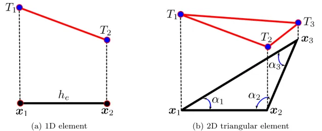
For future use, we provide the expressions of the elemental matricesM(e) and K(e) for piecewise linear elements in 1D and 2D cases. In the 1D case, the ‘elements’ are segments, as the one shown in Fig. 1a, the elemental matrices are given by
M(e)= ρcvhe
6
2 1 1 2
, K(e)= κ he
1 −1
−1 1
(31)
where he is the length of the element. In the 2D case, the elements are
triangles (see Fig. 1b). The general expressions forM(e) ([8], pp. 473) and
K(e) ([9], [10]) in this case are
M(e)=ρc v
σe 12
2 1 1 1 2 1 1 1 2
(32)
K(e)= κ
2
cot(α2) + cot(α3) −cot(α3) −cot(α2)
−cot(α3) cot(α1) + cot(α3) −cot(α1)
−cot(α2) −cot(α1) cot(α1) + cot(α2)
(33) whereσeis the triangle’s area and whereα
i denote the triangle’s inner angle
(a) 1D element (b) 2D triangular element
Figure 1: Linear elements in 1D and 2D
4.2. Thermodynamic Consistency Analysis
The question posed here is if the temperature solutions Th(x, t) gen-erated by the CGFE method, and defined in problem (Ph), are globally thermodynamically consistent. In order to answer this question, we need to reconstruct the thermodynamic tuple ΠPh = [T,e,s,q] associated to (Ph).
The reconstruction is straightforward. The thermodynamical tuple ΠPh is
equal to ΠP except that the temperature field, is not longer the exact
solu-tionT(x, t) but its CGFE approximation Th(x, t), so:
ΠPh = Π(Th) =
Th,e(Th),s(Th),q(Th) (34)
Now, having the corresponding tuple ΠPh = Π(Th) well defined, we can test
for global thermodynamic consistency of the CGFE solutions.
4.2.1. Consistency Analysis with respect to the First Law
Let us prove that the discrete solutions Th(x, t) are globally consistent with respect to the first law of thermodynamics. This is done in the following theorem.
Theorem 4.1. All discrete CGFE solutions Th(x, t) of the heat equation (P) are globally consistent with respect to the first law of thermodynamics. Proof. We need to prove that the termodynamical tuple ΠPh= Π(Th)
pro-duced by the solutionsTh always satisfies the global statement of the first law of thermodynamics, Eq. (5)(a). In other words, we need to prove that:
Z
Ω
for ΠPh = Π(Th).
The proof goes as follows. From the expression of specific energy eof ΠPh
given in Eq. (34), we have:
Z
Ω
ρe˙dv =
Z
Ω
ρ∂e(T
h)
∂t dv =
Z
Ω
ρcvT˙hdv (36)
where, for the last equality, we have used Eq. (8-(a). Now, using the expression for ˙Th given in Eq. (22)(b), we get that
Z
Ω
ρe˙dv=X
j Z
Ω
ρcvϕjdv
˙
Tj (37)
Using the partition of unity propertyP
iϕi = 1 , we get: Z
Ω
ρe˙dv =X
i X
j Z
Ω
ρcvϕiϕjdv
˙ Tj =
X
i X
j
MijT˙j (38)
where in the last equality we have used the definition of mass matrix M. Now, using Eq. (22)(c), we get that:
Z
Ω
ρe˙dv =X
i X
j
KijTj = X
j X
i
Kij !
Tj (39)
Finally, we prove the desired statement, Eq. (35), by noticing that the last term of the equations above is zero, because of the stiffness matrix property condition (27).
Note that the above theorem is valid for all solutions Th independently of the initial conditions and the mesh. The theorem proves that all solutions Th conserve total energy.
4.2.2. Consistency Analysis with respect to the Second Law
Now, we address the problem of determining if the CGFE solutions are globally consistent with respect to the second law of thermodynamics. Con-trary of what might be conjectured we will prove that not all obtained CGFE solutions are globally consistent with the second law of thermodynamics. In order to prove this we shall build particular cases where the second law statement, R
Ωρs˙dv > 0, is violated. In order, to perform this
Lemma 4.1. At any timet, the rate of change of total entropyS˙h =R Ωρs˙dv
associated to the CGFE solutions,Th(x, t), can be computed as sum of ele-mental contributions using the following general formula:
˙
Sh(t) =
Z
Ω
ρs(x, t)˙ dv =X
e
˙
Se(t) (40)
where:
˙
Se(t) =ρc v
Z
Ωe
Pne
je ϕje(x) ˙Tje(t)
Pne
keϕke(x)Tke(t)
dv (41)
wherekeandjedenote local indices of the basis functions ϕje that are active
in element e and where ne denote the total number of these functions, and where,Tje andT˙je denote the nodal temperature and nodal temperature rates
associated to those local indices, respectively.
Proof. Recall that the thermodynamic tuple ΠPh = Π(Th) associated to the
solutions Th of (Ph) is given in Eq. (34). From the expression of specific entropys of such equation, we have:
˙
Sh = Z
Ω
ρs˙dv =
Z
Ω
ρ∂s(T
h)
∂t dv =
Z
Ω
ρcv
˙ Th
Th dv (42)
where in the last equality we have used Eq. (8-(b). Now, using the expres-sions forTh and ˙Thgiven in Eqs. (22)(a-b) in the last term of the equations above we get that:
˙
Sh(t) =ρcv Z
Ω
˙ Th(x, t)
Th(x, t)dv =ρcv Z
Ω P
jϕj(x) ˙Tj(t) P
kϕk(x)Tk(t)
dv (43)
In the equations above, we have introduced the function arguments for help-ing the reader to understand what is behelp-ing computed. We have also made use thatρ and cv are assumed constants for simplicity. Note from Eq. (43)
that computing total entropy rate ˙Sh requires the computation of a rational
function having basis functions in the numerator and denominator. It is not possible to find an analytical expression for this integral. However, we can procced further and make use of finite element properties to decompose such integral as the sum of elemental entropy-rate contributions, ˙Se, along
the mesh elements Ωe. Then, performing this decomposition, Eq. (43) can be re-written as:
˙
Sh(t) =X e
˙
where
˙
Se(t) =ρcv Z
Ωe
˙ Th(x, t)
Th(x, t)dv =ρcv Z
Ωe
P
jϕj(x) ˙Tj(t) P
kϕk(x)Tk(t)
dv (45)
Then, keeping only the nodal basis functions ϕ that are active in each el-ement ‘e’, it follows that Eq. (45) can be rewritten as Eq. (41), which completes the proof.
Next, analytical expressions for the entropic elemental contributions ˙Se
will be obtained for the popular cases of piecewise linear basis functions in 1D and 2D, i.e., for segments and triangular elements. This formulae will be presented in the following two lemmas.
Lemma 4.2. At any timet, the rate of change of elemental entropyS˙e, for
piecewise linear 1D elements can be computed from the following formula:
˙
Se=ρc
vheND (a)
where
if T16=T2 (b)
N = (T1−T2)( ˙T1−T˙2) + (T2T˙1−T1T˙2) log[T2/T1]
D= (T1−T2)2
if T1=T2 (b)
N = ˙T1+ ˙T2
D= 2T1
(46)
where he is the lenght of element e, and where, T1, T2 and T˙1,T˙2 are the
nodal temperatures and the nodal rates of the 1D element, at such timet, as shown in Fig. 1a.
Proof. In the 1D case, the general formula for ˙Se, given in Eq. (41),
be-comes:
˙
Se=ρcv Z
he
ϕ1(x) ˙T1+ϕ2(x) ˙T2
ϕ1(x)T1+ϕ2(x)T2
dx=ρcv Z x2
x1
ϕ1(x) ˙T1+ϕ2(x) ˙T2
ϕ1(x)T1+ϕ2(x)T2
dx (47)
where local indices associated to elementeare used (see Fig. 1a). Now, the integral along the segment [x1, x2] can be mapped into a master segment,
[0,1], of unit lenght having local coordinatesu with vertices at u1 = 0 and
u2 = 1, so Eq. (47) can be re-written as:
Note that the nodal functions ϕ1 and ϕ2, in local coordinates u, become
ϕ1 = 1−u and ϕ2 = u, respectively. After analytical integration of the
RHS of Eq. (48), one obtains that ˙Se can be computed from Eq. (46). This
completes the proof.
Lemma 4.3. At any time t, the rate of change of elemental entropy S˙e,
for piecewise linear triangular elements can be computed from the following formula:
˙
Se=ρc v2σe
N1T˙1+N2T˙2+N3T˙3
D (49) where
if T1 6=T26=T3 6=T1
D= 2(T1−T2)2(T1−T3)2(T2−T3)2
N1 =−T1(T2−T3)2(−2T2T3+T1T2+T1T3) Log[T1]+
+T22(T1−T3)2(T2−T3) Log[T2]−T32(T1−T2)2(T2−T3) Log[T3]+
+T1(T1−T2)(T1−T3)(T2−T3)2
N2 =−T2(T1−T3)2(−2T3T1+T1T2+T2T3) Log[T2]+
+T12(T2−T3)2(T1−T3) Log[T1]−T22(T1−T2)2(T1−T3) Log[T3]
−T2(T1−T2)(T1−T3)2(T2−T3)
N3 = +T3(T1−T2)2(2T1T2−T1T3−T2T3) Log[T3]+
+T12(T2−T3)2(T1−T2) Log[T1]−T22(T1−T3)2(T1−T2) Log[T2]+
+T3(T1−T2)2(T1−T3)(T2−T3)
if T1 =T2=T3
D= 6T1, N1= 1, N2 = 1, N3 = 1
(50)
if T1 =T26=T3
D= 2(T1−T3)2(T1−T3)2
N1 = (1/2)(T1−T3) T12−4T1T3+ 3T32+ 2T32Log[T1/T3]
N2 = (1/2)(T1−T3) T12−4T1T3+ 3T32+ 2T32Log[T1/T3]
N3 = (T1−T3)(T12−T32−2T1T3Log[T1/T3])
if T1 =T36=T2
D= 2(T1−T2)2(T1−T2)2
N1 = (1/2)(T1−T2) T12−4T1T3+ 3T22−2T22Log[T2/T1]
N2 = (T1−T2) T12−T22+ 2T1T2Log[T2/T1]
N3 = (1/2)(T1−T2) T12−4T1T3+ 3T22−2T22Log[T2/T1]
if T1 6=T2=T3
D= 2(T1−T2)2(T1−T2)2
N1 = (T1−T2) T12−T22−2T1T2Log[T1/T2]
N2 = (1/2)(T1−T2) (T1−T2)(−3T1+T2) + 2T12Log[T1/T2]
N3 = (1/2)(T1−T2) (T1−T2)(−3T1+T2) + 2T12Log[T1/T2]
where he is the lenght of element e, and where, T1, T2 and T˙1,T˙2 are the
nodal temperatures and the nodal rates of the 1D element, at such timet, as shown in Fig. 1a.
Proof. In the 2D case, with triangular elements , Eq. (41) becomes:
˙
Se=ρcv Z
σe
ϕ1T˙1+ϕ2T˙2+ϕ3T˙3
ϕ1T1+ϕ2T2+ϕ3T3
da (52)
where, again, local elemental indices are used and where ϕi is the shape
function of nodei, located at vertexxi of the triangular element, as shown
in Fig. 1b), and where, {Ti,T˙i,i= 1,2,3} denote the corresponding nodal
temperatures and the nodal temperature-rates, at time t, at such nodal points. For the sake of simplicity assume that the local elemental index numbering is chosen so “node 1” has the minimun nodal temperature, that is to say: T1= min(T1, T2, T3). Note also thatT is absolute temperature, so
one must have thatT1, T2, T3 >0. Mapping the above integral into a master
triangular element having local coordinates (u, v) and vertices (0,0), (0,1) and (1,0), and using the expressions of the shape functions in terms of these local coordinates, one has that the elemental entropy can be computed as:
˙¯
Se =ρcv2σe Z 1
0
Z 1−u
0
(1−u−v) ˙T1+uT˙2+vT˙3
(1−u−v)T1+uT2+vT3
dudv (53)
whereσe is the area of the triangular element Ωe. Then the above integral can be written as:
˙¯
Se= ρcv2σ
e
T1 Z 1
0
Z 1−u
0
(1−u−v) ˙T1+uT˙2+vT˙3
(1−u−v) +u(T2/T1) +v(T3/T1)
dudv (54)
From Eq. (54), it follows that except by a scaling factor, the elemental entropy rate depends on the relative values of nodal temperatures. After analytical integration of the RHS of Eq. (54), one obtains that ˙Se can be
computed from Eq. (47). This completes the proof.
From the above Lemmas, it follows that, at any timet, the total entropy rate ˙Sh = R
Ωρs˙dv of any discrete finite element solution Th(x, t) can be
computed by summation of the elemental contributions ˙Se(t) calculated
using Eq. (46) for 1D linear elements and Eq. (49) for linear triangular elements. 4.
Now, the above lemmas will be used to build simple examples which will prove that the CGFE method is not entropically consistent. The examples will prove that the CGFE method can generate discrete solutions Th(x, t)
that violate the global statement of the second law of thermodynamics given in Eq. (5(b), which asserts that total entropy must always satisfy that
R
Ωρs˙dv>0.
4.2.2.1 Failure Examples 1D Case
Consider the case of heat conduction in a one-dimensional material bar of unit lenght L = 1 whose end points are located at x = 0 and x = 1, as the one shown in red in Fig. 2. Assume for simplicity that the bar is made of a material with unit propertiesρ,cv,κ= 1. Assume the bar is fully
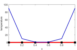
isolated from the exterior. Suppose the bar is discretized by a mesh of 5 equal elements and 6 nodes, and, assume the initial temperature distribution in the bar is given byT = [T1, T2. . . , T6]> = [90,10,1,1,10,90]>, as shown in Fig.
2. The instantaneous vector of nodal temperature rates T˙ is determined by the CGFE method through Eq. (22)(c). The rate of change of total entropy ˙Sh associated to such evolutionary state can be computed using
Eqs. (40) and (46). The resulting value is ˙Sh = −24.67. This negative
value indicates a violation of the second law of thermodynamics (??). This proves that the CGFE is not entropically consistent for linear elements in 1D. It must be pointed out that not all discrete solutions produced by the CGFE method violate the second law, only some of them do. For example, if one runs an experiment where different vectors of nodal temperatures T = [T1, T2. . . , T6]> are generated by choosing the nodal temperatures from
the set of four possible values Ti = {1, 10, 40, 90}, i = 1 : 6, only 5
values of T (out of the 4096 cases) will generate a temperature evolution that violate the condition ˙Sh ≥ 0. Also, it is important to note that the
violation of entropy not necessarily will occur at all times. For example, if the time-evolution of nodal temperatures (see Fig. 3a) is computed for subsequent times for the case of the initial condition T shown in Fig. 2, it can be observed from Fig. 3b that the entropy rate will violate the second law of thermodynamics only at the first times of the simulation. Of course, such violation will have an impact in the future temperature behavior. At least one anomalous behavior can be detected in the predicted evolution of nodal temperatures shown in Fig. 3a: at initial times, the nodes that have the minimum temperature (Ti = Tmin = 1, i = 3,4), instead of showing
Figure 2: Heat conduction in an isolated 1D bar shown in red color. The bar is discretized by 5 elements with an initial temperature distribution shown in blue color
(a) Evolution of nodal temperaturesT(t) (b) Evolution of total entropy rate ˙Sh(t)
Figure 3: Temperature and total entropy rate time-evolution predicted by the CGFE method in an isolated 1D bar for the initial temperature distribution shown in Fig. 2
.
may speculate that the negative values of ˙Sh may indicate the presence of
non-physical, reversed, heat flows occurring inside the domain due to the discretization process. This is in agreement with a recent result [4].
4.2.2.1 Failure Examples 2D Case
Consider the following heat conduction problem in a body with quad-rangular shape, as the one shown in Fig. ??. Assume the body is fully isolated: it does not received nor give up heat from the exterior. For simplicity, assume that the body is made of a material with unit proper-ties ρ, cv, κ = 1. Assume the body is discretized by a mesh of 12 equal
triangular elements and 12 nodes, as shown in Fig. ??. The triangular elements conforming the mesh have inner angles given by: α1 = 20 deg,
α2 = 150 deg andα3 = 10 deg. The nodal coordinatesxi = (xi, yi) are given
temperatures is defined byT = [T1, T2. . . , T12]>. Given a vectorT, the
vec-tor of nodal temperature rates T˙ can be found from Eq. (22)(c). With the values of {T,T˙}, the total entropy rate ˙Sh of the discrete solution can be
computed from Eqs. (40) and (49). Now, let us run a numerical experiment where values of ˙Sh will be computed for different initial temperature states
T. For this purpose, let us assign each nodal temperature Ti, i = 1, ..,12
a temperature value of the following set {1, 10, 50}, considering all possi-ble permutations of resulting vectors T. With 12 nodes there are a total number of 312 = 531441 possible permutations. For each permutation, a value of T is set, T˙ can be determined, and ˙Sh can be computed to verify
that the second law of thermodynamics is satisfied ( ˙Sh ≥0). If CGFE
dis-cretizations were fully thermodynamically consistent, such condition should be satisfied for all permutations. The results of the experiment show that, like in the 1D case, some discrete solutions violate the second law ( ˙Sh<0).
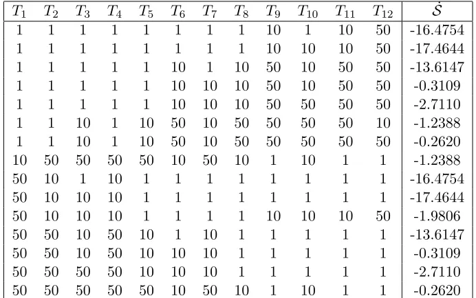
For the present experiment, 15 entropically inconsistent solutions were de-tected. They are given in Table 1. The corresponding values of negative entropy rates are shown in the last column. In Fig. ??, the distribution of temperatures in the quadrangular body are shown for the entropically in-consistent case defined in the 12th-row of Table 1. The experiments proves that the CGFE method is not consistent with respect to the second law of thermodynamics for linear triangular elements.
5. Conclusions
T1 T2 T3 T4 T5 T6 T7 T8 T9 T10 T11 T12 S˙
1 1 1 1 1 1 1 1 10 1 10 50 -16.4754
1 1 1 1 1 1 1 1 10 10 10 50 -17.4644
1 1 1 1 1 10 1 10 50 10 50 50 -13.6147
1 1 1 1 1 10 10 10 50 10 50 50 -0.3109
1 1 1 1 1 10 10 10 50 50 50 50 -2.7110
1 1 10 1 10 50 10 50 50 50 50 10 -1.2388
1 1 10 1 10 50 10 50 50 50 50 50 -0.2620
10 50 50 50 50 10 50 10 1 10 1 1 -1.2388
50 10 1 10 1 1 1 1 1 1 1 1 -16.4754
50 10 10 10 1 1 1 1 1 1 1 1 -17.4644
50 10 10 10 1 1 1 1 10 10 10 50 -1.9806
50 50 10 50 10 1 10 1 1 1 1 1 -13.6147
50 50 10 50 10 10 10 1 1 1 1 1 -0.3109
50 50 50 50 10 10 10 1 1 1 1 1 -2.7110
50 50 50 50 50 10 50 10 1 10 1 1 -0.2620
Table 1: Nodal temperature configurations T producing violation of the second law of
thermodynamics ( ˙Sh
<0)
For linear triangular elements in 2D, this does not seem to be enough. In this case, meshes with special types of triangular shapes might be necessary. The authors think that the issue discussed in this paper might be connected with the observation that CGFE discretizations violate, nodally, the Clausius’s Postulate of the second law which has been reported in a recent work [4]. In this sense, the global inconsistency may be a measure of the existence of non-physical reversed heat flows produced by the discretization procedure. Finally, it must be pointed out that the mathematical background presented here is general and could be used to explore the thermodynamic consistency of other types of elements, such as quadrangular or tetrahedral elements, as well, as other variants of finite element formulations.
References
duced by Laplace formulations, Computer Methods in Applied Mechan-ics and Engineering 197 (2008) 1703–1759.
[3] T. J. R. Hughes, G. Engel, L. Mazzei, M. G. Larson, The continu-ous galerkin method is locally conservative, Journal of Computational Physics 163 (2000) 467-488.
[4] A. Limache, S. Idelsohn, On the issue that finite element discretiza-tions violate, nodally, Clausius’s postulate of the second law of thermo-dynamics, Advanced Modeling and Simulation in Engineering Sciences 3 (13) (2016) 1–18.
[5] M. Gurtin, E. Fried, L. Anand, The Mechanics and Thermodynamics of Continua, Cambridge University Press, 2010.
[6] C. Truesdell, Rational Thermodynamics, Springer-Verlag, 1984. [7] M. Larson, F. Bengzon, The Finite Element Method: Theory,
Imple-mentation and Applications, Vol. 10 of Texts in Computational Science and Engineering, Springer, 2013.
[8] O. Zienkiewicz, R. Taylor, The Finite Element Method - Fifth Edition, Vol. 1, Butterworth-Heinemann, 2000.
[9] A. Draganescu, T. F. Dupont, L. R. Scott, Generalized local maxi-mum principles for finite-difference operators, Math. of Comp. 27 (124) (2004) 685–718.