Article
On the Wake Properties of Segmented Trailing Edge
Extensions
Sidaard Gunasekaran1, Daniel Curry2
1 2 3 4
5 6 7 8
9 10 11 12
13 14
1 AssistantProfessor,DepartmentofMechanicalandAerospaceEgnineering,UniversityofDayton;
2 UndergraduateStudent,DepartmentofMechanicalandAerospaceEngineering,UniversityofDayton;
* Correspondence:[email protected];Tel.:+1-937-229-5345
Abstract: Changesintheamountandthedistributionofmeanandturbulentquantitiesinthefree shearlayerwakeofa2DNACA0012airfoilandAR4NACA0012wingwithpassivesegmented rigidtrailingedge(TE)extensions wasinvestigatedattheUniversityofDaytonLowSpeedWind Tunnel (UD-LSWT).TheTE extensions were intentionally placedat zero degreeswith respectto thechordlinetostudytheeffectsofsegmentedextensionswithoutchangingtheeffectiveangleof attack.Forcebasedexperimentswasusedtodeterminethetotalliftcoefficientvariationofhtewing withsevensegmentedtrailingedgeextensionsdistributedacrossthespan. Thesegmentedtrailing edgeextensionshadnegligibleeffectofliftcoefficientbutshowedmeasurabledecrementinsectional and totaldragcoefficient.I nvestigationo ft urbulentq uantities( obtainedt hroughP articleImage Velocimetry(PIV))suchasReynoldsstress,streamwiseandtransverseRMSinthewake, reveala significantdecreaseinmagnitudewhencomparedtotheb aseline.Thedecreaseinthemagnitude of turbulent parameters was supported by thechanges in coherent structures obtained through two-pointcorrelations. Apartfromthereductionindrag,thelowerturbulentwakegeneratedby theextensionshasimplicationsinreducingstructuralvibrationsandacoustictones.
Keywords:TrailingEdgeExtensions;DragReduction;CoherentStructures.
15
1. Introduction
16
The ideology of application of trailing edge extensions on streamlined bodies to affect wing
17
performance dates to WWII where NACA investigated the use of TE extensions on propeller blades
18
to change the camber and effective angle of attack of propeller sections [1]. Based on the extension
19
geometry, orientation and the airfoil, the design CL can be matched with the operating conditions
20
of the propeller sections to obtain an optimum pressure distribution. Theodorsen and Stickle [1]
21
derived theoretical expressions for the changes in effective angle of attack of the wing as a function
22
of extension length and angle using thin airfoil theory. But validation of theoretical work with
23
experimental work was not done till later. In 1989, Ito [2] performed experimental investigations
24
to study the effect of trailing edge extensions on Göttingen 797 and Wortmann FX 63-137 airfoils used
25
on earlier STOL aircraft, at Reynolds numbers between 300,000 and 1,000,000. The extensions, when
26
placed along the camber-line, significantly increased the CL max and L/D for Gö797 but didn’t have
27
any effect on the Wortmann airfoil due to its high camber and a complicated curved lower surface.
28
This result indicated that the effectiveness of the TE extensions depend significantly on the airfoil
29
profile.
30
This sensitivity on the effectiveness of TE extensions on the airfoil profile is due to angle of the
31
free shear layer wake and characteristic turbulence. Most airfoils experience vortex shedding at the
32
2 of 21
trailing edge resulting in the loss of total pressure, hence drag increase. Similar to a cylinder, the
33
vortex shedding behind a wing is a function of Reynolds number as shown in experiments done by
34
Yarusevych et al [3]. They determined that the roll-up of vortices in the separated shear layer play a
35
key role in the flow transition to turbulence. The relationship between the flow separation and vortex
36
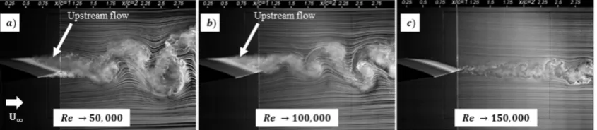
shedding in an airfoil can be clearly seen in Figure1taken from Yarusevych et al. [3] where the smoke
37
released downstream of the wing is seen upstream on top of the wing.
38
Figure 1. Shedding of vortices from the trailing edge of NACA 0025 airfoil at different Reynolds
numbers. (adapted from Yarusevych [3])
Figure1shows prominent turbulent wake vortex shedding due to the separated upper surface
39
shear layer. Huang and Lin [4] and Huang and Lee [5] performed experiments on NACA 0012 airfoil
40
and reported that the vortex shedding is only observed at lower Reynolds numbers where boundary
41
layer separation occurs without reattachment. Yarusevych et al. [3] amended this result and proved
42
that vortex shedding occurs even after boundary layer attaches to the surface at higher Reynolds
43
number as shown in Figure 1c and that the vortex shedding varies linearly with the Reynolds number.
44
The vortex shedding is also found to be a function of trailing edge geometry. Guan et al. [6]
45
experimented with multiple beveled trailing edge geometries and showed that even subtle changes
46
in geometry can result in substantial changes in wake signatures. The vortex shedding was found to
47
be greater at the sharp trailing edge when compared to the rounded trailing edges. But even with
48
the smooth trailing edge, the turbulent coherent structures were found to convect without distinct
49
separation points into the wake which complements the result from Yarusevych et al.[3].
50
Therefore, the effectiveness of the TE extensions depends on the length and angle of the TE
51
extension, the airfoil section, the effective angle of attack of the wing, chord based Reynolds number
52
and trailing edge geometry. All these parameters affect the vortex shedding behind the wing which
53
influences the parasite drag experienced by the wing. The parasitic drag contribution on airplanes
54
during cruise is in the order of 50% of the total drag [7]. The streamwise pressure gradient created
55
by the periodic shedding of vortices initiates on-body flow separation resulting in higher drag,
56
undesirable structural vibrations and higher acoustic levels.
57
The current study is aimed at investigating the sensitivity of the segmented TE extensions on
58
the amount and distribution of vorticity and the turbulent parameters in the free shear layer wake.
59
However, some techniques used to mitigate vortex shedding is shown below.
60
1.1. Vortex Mitigation Techniques
61
Most of the parasitic drag reduction methods on a wing is targeted at keeping the boundary layer
62
attached and delaying the transition. A slew of active and passive flow control techniques involving
63
laminar flow control, wall cooling, hybrid laminar flow control, active wave suppression, use of
64
riblets, vortex generators, large eddy breakup devices, surface geometry effects such as streamwise
65
and transverse curvatures and microgrooves, synthetic boundary layer, etc were used to prevent
66
boundary layer transition and separation. But when compared to the number of methods available to
67
mitigate vortex shedding from bluff bodies such as cylinders, trucks, cars, etc. the number of methods
68
available to mitigate vortex shedding from streamlined bodies are minimal.
69
Preprints (www.preprints.org) | NOT PEER-REVIEWED | Posted: 5 August 2018 doi:10.20944/preprints201807.0266.v2
One of the popular methods to mitigate the influence of vortex shedding from wing is the use
70
of Gurney flaps or divergent trailing edges. Gurney flap is an extension of the trailing edge in the
71
direction perpendicular to the chord. The use of Gurney flap generates a favorable streamwise
72
pressure gradient at high angle of attack and is known to shift the location of the separation from
73
the leading edge to the quarter chord location while at the same time increasing lift on the main
74
airfoil profile (Stanewsky [8]). A finite pressure differential is carried to the trailing edge and is
75
sustained by a vortex shedding induced base pressure on the downstream face of the flap. Numerous
76
computational and experimental work have been done to study the effect of length and angle of
77
Gurney flaps on vortex shedding. (Neuhart and Pendergraft [9], Jang and Ross [10], Storms and Jang
78
[11], Traub [12]). But these flaps are usually more effective at higher angles of attack where the flow
79
separates and actually generates higher drag as expected in areas where flow is not separated.
80
The disadvantage of higher drag using Gurney flaps at lower angles of attack can be overcome
81
by having a static extended trailing edge (SETE) or flexible extended trailing edge (FETE).
82
Figure 2. a) NACA 0012 wing with static extended trailing edge. b) Variation of aerodynamic
efficiency with coefficient of lift for baseline, Gurney and SETE configurations. The SETE configuration yielded better aerodynamic efficiency than the Gurney flap (adapted from Lui et al. [13]).
Lui et al. [13] attached a thin flat plate at the trailing edge of NACA 0012 airfoil made of
83
aluminum and Mylar and determined the changes in the airfoil efficiency as a function of angle of
84
attack and compared it with the measurement made from Gurney flap (Figure2). SETE showed a
85
larger lift increase at a smaller drag penalty better than a Gurney flap since the SETE was in between
86
the wake of the main airfoil. SETE shows improvement in lift characteristics across the range of angles
87
of attack when compared to Gurney flaps where the lift improvement is seen only at higher angles
88
of attack. Lui et al. [13] also determined the aeroelastic deformation for aluminum (less than 1%)
89
and Mylar (13%) and postulated that MEMS microphones can be embedded in the SETE which will
90
change and react to surroundings. A similar approach is used in this research but instead of using
91
a SETE, a segmented TE extensions was used to conserve weight and reduce drag forces on a wing.
92
Segmented TE extensions can also act as control surfaces which was implemented by Lee and Kroo
93
[14] where they placed microflaps or Miniature Trailing Edge Effectors (MiTE) on the trailing edge of
94
the high aspect ratio wings (Figure3) to suppress flutter through dynamic deflection. With this type
95
of controller, they were able to increase the flutter speed by 22%.
4 of 21
The background research indicates that extended trailing edges could be effective in reducing
97
drag and increasing lift in wings and TE extensions could lead to drag reduction and control flutter
98
speed and could possibly act as control surfaces. A major disadvantage of TE extension is that it
99
contributes to overall weight of the aircraft. This research explores the use of segmented TE extensions
100
as a means to increase the aerodynamic efficiency and reduce the turbulent fluctuations in the wake
101
of the wing.
102
Figure 3.Array of MiTEs (adapted from Lee and Kroo [14])
2. Experimental Setup
103
2.1. Wind Tunnel
104
All the experiments were conducted at the University of Dayton Low Speed Wind Tunnel
105
(UD-LSWT). The UD-LSWT has a 16:1 contraction ratio, 6 anti-turbulence screens and 4
106
interchangeable 76.2cm x 76.2cm x 243.8cm (30” x 30” x 96”) test sections. The test section is
107
convertible from a closed jet configuration to an open jet configuration with the freestream range
108
of 6.7m/s (20 ft/s) to 40m/s (140 ft/s) at a freestream turbulence intensity below 0.1% measured
109
by hot-wire anemometer. All the experiments mentioned in the paper were done in the open jet
110
configuration where an inlet of 76.2 cm x 76.2 cm opens to a pressure sealed plenum. The effective
111
length of the test section in the open jet configuration is 182cm (72”). A 137cm x 137cm (44” x 44”)
112
collector collects the expanded air on its return to the diffuser. A photo of the UD-LSWT open jet
113
configuration is shown in Figure4. The velocity variation for a given RPM of the wind tunnel fan is
114
found using a Pitot tube connected to an Omega differential pressure transducer (Range: 0 – 6.9 kPa).
115
Figure 4.University of Dayton Low-Speed Wind Tunnel (UD-LSWT) in the open-jet configuration.
Preprints (www.preprints.org) | NOT PEER-REVIEWED | Posted: 5 August 2018 doi:10.20944/preprints201807.0266.v2
2.2. Test Model
116
A NACA 0012 semi-span wing with 20.32 cm span (b) and 10.16 cm chord (c) was designed in
117
SolidWorks with capability to attach multiple TE extensions as seen in Figure5. The wing was then
118
3D printed using Stratasys uPrint SE Plus printer at the University of Dayton. The wing model uses
119
two pieces to clamp the TE extensions to the main wing. The design allows for multiple TE extensions
120
to be mounted. Seven segmented plexiglass TE extensions with thickness (t) of 1 mm, length (l) of
121
2.54 cm (l/c = 0.25) and a width (d) of 0.635 cm (d/c = 0.0625) were used. With the trailing edge
122
extensions, the surface area of the wing was increased by 11% when compared to the baseline.
123
Figure 5.SolidWorks model of AR 4 NACA 0012 wing with TE extensions.
2.3. Force Based Experiment
124
Force based experiments were performed on the NACA 0012 semispan model with and without
125
the segmented TE extensions at a Reynolds number of 200,000 (Test Matrix shown in Table1). The
126
models were tested at an angle of attack range from -15◦to +15◦. Two trials of the same experiment
127
were done with increasing and decreasing the angle of attack to check for hysteresis. The schematic
128
of the force based test setup is shown in Figure6.
129
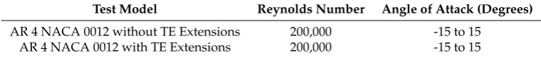
Table 1.Test Matrix for the force based experiments.
Test Model Reynolds Number Angle of Attack (Degrees)
AR 4 NACA 0012 without TE Extensions 200,000 -15 to 15 AR 4 NACA 0012 with TE Extensions 200,000 -15 to 15
An ATI Mini-40 force transducer was secured underneath the wing at the quarter chord location
130
which interfaced with the Griffin motion rotary stage to change the angle of attack. The rotary stage
131
was controlled using the Galil motion software. The schematic of the test setup is shown in Figure6.
132
The root of the wing was made to be in alignment with the splitter plate.
6 of 21
Figure 6.Schematic of the force based experiment test setup for NACA 0012 semispan model with TE
extensions. Similar setup was used for NACA 0012 wing without TE extensions as well.
2.4. Force Transducer
134
An ATI Industrial Automation Mini-40 (www.ati-ia.com) sensor was used to determine the wing
135
lift and drag coefficients. The specifications for the Mini – 40 sensor are shown in Table 2. The normal
136
and axial force was measured using the X and Y axes of the sensor. The sampling rate during data
137
acquisition from the Mini-40 was 100 Hz. To make sure the sampling rate doesn’t bias the force based
138
experiments due to vortex shedding frequency, force experiments were conducted at the Reynolds
139
number of 135,000 and 200,000 and the lift coefficient variation was compared.Tare values were taken
140
before and after each test, and then the average of the two tares are subtracted from the normal and
141
axial force readings.
142
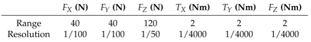
Table 2.Test Matrix for the force based experiments.
FX(N) FY(N) FZ(N) TX(Nm) TY(Nm) FZ(Nm)
Range 40 40 120 2 2 2
Resolution 1/100 1/100 1/50 1/4000 1/4000 1/4000
2.5. PIV Setup
143
Streamwise Particle Image Velocimetry (PIV) was conducted in the free shear layer of the NACA
144
0012 wall-to-wall model with and without the segmented TE extensions. Two end plates were
145
installed at the wingtips to prevent the rollup of wingtip vortex and reduce three dimensionality. The
146
PIV measurements were obtained using a Vicount smoke seeder with glycerin oil and a 200 mJ/pulse
147
Nd: YAG frequency doubled laser (Quantel Twins CFR 300). A Cooke Corporation PCO 1600 camera
148
(1600 x 1200 pixel array) with a 105 mm Nikon lens was used to capture the images. One plano-convex
149
lens and one plano-concave lens were used in series to convert the laser beam into a sheet. The
150
laser and the camera were triggered simultaneously by a Quantum composer pulse generator. In
151
each test case, over 1000 image pairs were obtained and processed using ISSI Digital Particle Image
152
Velocimetry (DPIV) software. A total of 2 iterations were performed during PIV processing with
153
64-pixel interrogation windows in the first iteration and 32-pixel interrogation windows in the second
154
iteration. Both the streamwise and cross-stream PIV interrogations were conducted a Reynolds
155
number of 135,000. The test matrix for the PIV experiment is shown in Table 3. The schematic of
156
Preprints (www.preprints.org) | NOT PEER-REVIEWED | Posted: 5 August 2018 doi:10.20944/preprints201807.0266.v2
the PIV test setup is shown in Figure7a. The uncertainty of the velocity measurements from the PIV
157
setup was calculated to be 0.1m/s
158
Table 3.Test Matrix for Free Shear Layer (FSL) PIV interrogation
Test Model Angle of Attack (Degrees) Interrogation Location
AR 4 NACA 0012 without TE Extensions 0,2,4,6,8 Behind TE AR 4 NACA 0012 with TE Extensions 0,2,4,6,8 Behind TE Extension
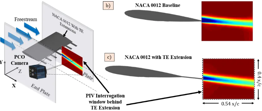
In the baseline case, the interrogation window was placed near the trailing edge of the wing as
159
shown in Figure 7b to determine the vortex shedding and the momentum deficit. In the wing with
160
the segmented TE extensions, the interrogation window was placed at the trailing edge of the TE
161
extension as shown in Figure 7a and 7c. Nikon 105 mm lens was used in the streamwise PIV case
162
which gave a spatial resolution of 292 pix/cm in both axes. The size of the field of view was 5.5 cm x
163
4.1 cm which gave a magnification factor of 0.21. TheδTfor the images were set to obtain an average
164
particle displacement of 8-10 pixels in the wake of the wing.
165
Figure 7.a) Schematic of the PIV test setup for the NACA 0012 wing with TE extensions. Similar setup
is used for the baseline wing. The PIV interrogation window for (b) the baseline case was located at the TE and (c) for the wing with TE extension, it was location at the trailing edge of TE
3. Influence of Reynolds number
166
Since the Reynolds numbers chosen for this study (200,000 and 135,000) falls within the
167
sub-critical and transitional regime, the influence of viscous effects on the aerodynamic coefficients
168
must be quantified. Spedding and McArthur [15] found a functional relationship between lift curve
169
slope and the Reynolds number between the order of 104and 105asCL =2πReβwhereβexponents
170
have the value of 0.19 for a 2D airfoil. But the Reynolds number influence of the coefficient of lift in
171
the moderate Reynolds numbers between 100,000 and 600,000 is less explored experimentally.
8 of 21
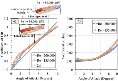
Figure 8.Comparison of a) lift coefficient b) drag coefficient at different Reynolds numbers.
However, the viscous effects on the aerodynamic coefficients can be determined through viscous
173
XFOIL simulation. Figure 8 shows the coefficients of lift and drag obtained from viscous flow
174
simulation in XFOIL for NACA 0012 at two Reynolds numbers considered in this study. The lift
175
coefficient deviates from the theoretical 2pi prediction at all angles of attack. This deviation is traced
176
to the movement of the separation point from the trailing edge of the airfoil and the formation of
177
laminar separation bubble. DNS simulations at a Reynolds number of 50,000 from I.Rodríguez et
178
al.[16] showed the presence of laminar separation bubble and the vortex breakdown at the end of the
179
bubble because of Kelvin-Helmholtz mechanism. The separation point moves towards the leading
180
edge with increase in angle of attack. The departure of the lift curve slope from the inviscid theory
181
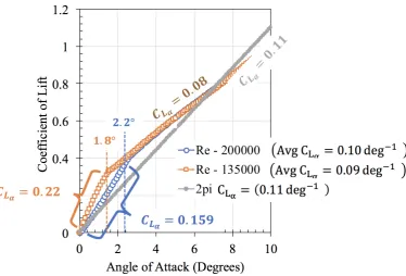
can be quantified through lift curve slope as shown in Figure9.
182
There is a change in the lift curve slope around 2◦angle of attack for both the Reynolds number
183
cases. But at angles of attack greater than 2◦, the lift curve slope (CLα) stays constant at 0.08deg−1.
184
On an average, the entire lift curve slope of the NACA 0012 at a Reynolds number of 135,000 is
185
around 0.09deg−1 and at a Reynolds number of 200,000, it is around 0.1deg−1 which deviates from
186
the lift curve slope of 2pi by 18% and 9% respectively. But irrespective of the viscous effects, the lift
187
curve remains linear. And with the relatively smaller percent difference between the theoretical and
188
simulated lift curve slope, the relationship between induced drag and the lift coefficient is expected
189
to remain the same.
190
Even though different Reynolds numbers were used for force-based testing and PIV, the lift and
191
drag characteristics of the NACA 0012 are the same as evidenced from the simulated results shown
192
in Figure9. After 2◦angle of attack, the lift coefficient from the two different Reynolds numbers is
193
identical. The drag coefficient also shows similar behavior and magnitude at two different Reynolds
194
numbers as well. Therefore, it can be concluded that there are no significant changes in the flow
195
characteristics over the NACA 0012 at the two different Reynolds numbers considered for this study.
196
Preprints (www.preprints.org) | NOT PEER-REVIEWED | Posted: 5 August 2018 doi:10.20944/preprints201807.0266.v2
Figure 9.Comparison of a) lift coefficient b) drag coefficient at different Reynolds numbers.
4. Results
197
4.1. Force-Based Experimental Results
198
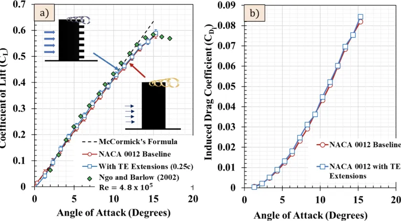
The coefficient of lift variation with angle of attack is shown in Figure10for the Reynolds number
199
of 200,000 for both the baseline case and the wing with TE extensions. The coefficient of lift variation
200
is compared with the theoretical lift coefficient variation given by McCormick’s formula (McCormick
201
[17]). According to McCormick’s formula, the lift curve slope depends on the aspect ratio by,
202
a= dCL
dα =a0
AR AR+2 ARAR++42
(1)
wherea0=2π, according to thin airfoil theory andARis the aspect ratio of the wing. The best fit line
203
of the lift curve gives an effective aspect ratio of 2 which is smaller than the intended aspect ratio of
204
4. The reduction in effective aspect ratio could be due to the wing-splitter plate interface contributing
205
to three dimensionality of the flow. The baseline results shows good match with the results from Ngo
206
and Barlow [18] for a Reynolds number of 480,000 for AR 2. The added 11% surface area was taken
207
into account in the calculation of lift from the wing with the TE extensions case. The comparison of
208
lift coefficient magnitude between the baseline and the wing with TE extensions shows almost no
209
variations as a function of angle of attack. Any changes in lift coefficient falls between the uncertainty
210
band of the sensor as indicated by the error bars.
10 of 21
Figure 10.a) Variation of Coefficient of Lift with angle of attack for baseline wing and wing with TE
extensions. The lift curve slope shows similar variation with negligible differences between the two cases. b) Variation of coefficient of induced drag for both cases.
The differences in lift is used to calculate the differences in the induced drag. The induced drag
212
was found by,
213
CD Induced= C
2 L
πeAR (2)
whereeis the span efficiency andARis the aspect ratio. The span efficiency of the baseline and wing
214
with TE extensions was found using the lift curve slope equation from thin airfoil theory (Equation
215
3).
216
a= a0
1+ a0 πeAR
(3)
whereais the lift curve slope of the finite wing anda0=2π. From Equation 3, the span efficiency for
217
the baseline was 0.69 for both the cases since they have the same lift curve slope. The wing with TE
218
extensions shows higher induced drag coefficient across all angles of attack (Figure10b). At 14 angle
219
of attack, the induced drag shows a 6% increase in the wing with TE extensions when compared
220
to the baseline. At lower angles of attack, the differences in the induced drag between two cases
221
is not resolvable due to the uncertainty limit of the ATI mini-40 sensor. Because drag is an order
222
of magnitude less than the lift, the sensor was not capable of measuring the differences in the drag
223
forces between the two cases. Therefore, streamwise Particle Image Velocimetry (PIV) was used to
224
determine the momentum deficit and the parasitic drag of the wing configurations. The results from
225
the PIV are discussed in the section below.
226
4.2. Momentum Deficit
227
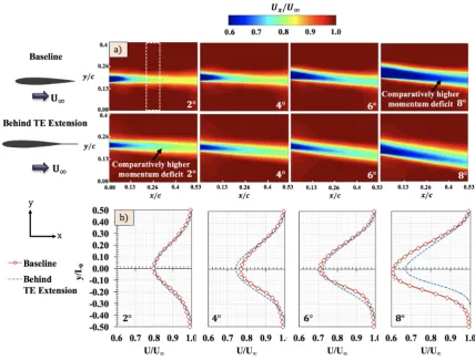
The streamwise velocityUX contour obtained behind the TE extension and behind the trailing
228
edge of the baseline wing is shown in Figure11a. The momentum deficit increases with increase in
229
angle of attack as expected for the both cases. However, subtle differences can be observed in the
230
momentum deficit between the two cases. At a 2◦angle of attack, the momentum deficit behind the
231
TE extension in greater than the momentum deficit behind the trailing edge of the wing. This could
232
Preprints (www.preprints.org) | NOT PEER-REVIEWED | Posted: 5 August 2018 doi:10.20944/preprints201807.0266.v2
be due to increased skin friction drag due to the presence of the TE extension. As the angle of attack
233
increases, the different trend is observed. At 4◦and 6◦angle of attack cases, the differences between the
234
two cases are hard to observe since the contours look almost similar. However, at 8◦angle of attack,
235
lower momentum deficit can be observed behind the TE extension when compared to the baseline.
236
This shows that the TE extension reduced the pressure drag of the wing.
237
Figure 11. a) Streamwise velocity contours in FSL behind the trailing edge of the NACA 0012 wing
and behind the TE extension b) Momentum deficit profiles at different angles of attack for both cases. The momentum deficit behind the TE extension is lower at higher angles of attack when compared to the baseline.
These observations are more apparent in the momentum deficit profiles shown in Figure11b.
238
The profiles were taken by averaging 10 data columns in the center of the field of view as highlighted
239
in Figure11. This region was chosen to avoid any influence of the distortion and spherical aberration
240
in the corners of the field of view. The normalized streamwise velocity is plotted against the
241
normalized wake-half widthy/L0whereL0is the wake half-width which is considered as the location
242
of 99%U∞. The profiles indicate that the momentum deficit at 2◦and 4◦angles of attack between
243
the two cases are similar. At 6◦and 8◦angle of attack however, clear differences between the two
244
cases can be seen. The momentum deficit behind the TE extension is clearly lower than the baseline.
245
The momentum deficit profiles shown in Figure11b was used to determine the total parasitic drag
246
coefficient of the baseline NACA 0012 wing and the wing with TE extensions. The total parasitic
247
drag coefficient of the wing was found by integrating the sectional drag coefficient along wingspan.
248
The sectional drag coefficient behind the trailing edge and the TE extension was determined by the
249
momentum deficit equation,
12 of 21
CD= ρU
2 ∞
q∞S
Z Ux
U∞
1− Ux U∞
dy (4)
where ρ is the density, U∞ is the freestream velocity and q∞ is the dynamic pressure, Ux is the
251
streamwise velocity andSis the surface area of the wing. The momentum deficit equation represents
252
the loss of momentum in the wake due to the presence of the wing in the flow. According to Newton’s
253
second law, by determining the reduction in the freestream momentum due to the presence of the
254
wing, the total drag of the wing can be estimated. The derivation of the momentum deficit principle
255
is detailed in Anderson [19]. The drag coefficient variation with angle of attack is shown in Figure
256
12. As expected, the drag coefficient behind the trailing edge varies non-linearly with the angle of
257
attack for both cases. The magnitude of the drag coefficient behind the TE extension is lower than
258
the baseline at all angles of attack. Even though the momentum deficit profiles in Figure11b look
259
similar for both the cases at lower angles of attack, the TE extension case has a higher chord length
260
and surface area when compared to the baseline case. Therefore, for a similar normalized momentum
261
deficit profile, the coefficient of drag is lower in the wake behind the TE extension.
262
Figure 12. Variation of coefficient drag estimation behind the trailing edge and behind TE extension
a function of angle of attack. The estimated drag coefficient behind the TE extension is lower than the drag coefficient behind the hole.
The differences in the sectional coefficient of drag increases with increase in angle of attack from
263
8% at 2◦to 12% at 8◦. To determine the total parasitic drag coefficient of the entire wing with and
264
without TE extensions, a theoretical distribution of the sectional drag coefficient is plotted in Figure
265
13 for 8-hole wing using the drag coefficient values obtained from the momentum integral. The
266
sections of the wing with the TE extension has a lower drag coefficient than trailing edge as observed
267
in Figure12. The theoretical drag coefficient distribution increases with angle of attack as expected.
268
The total drag coefficient of the wing was found by integrating the sectional drag coefficient
269
along the span of the wing. The net parasitic drag coefficient of the NACA 0012 baseline wing and
270
the wing with TE extensions are shown in Figure14a for multiple angles of attack. The total parasite
271
drag of the wing with TE extensions is lower than the NACA 0012 baseline wing across all angles of
272
attack. Adding the induced drag found from force based experiment and parasitic drag data found
273
from PIV, the total drag coefficient for the baseline and the wing with TE extension is shown in Figure
274
14b. The total drag for the wing with TE extensions is also lower when compared to the baseline at
275
Preprints (www.preprints.org) | NOT PEER-REVIEWED | Posted: 5 August 2018 doi:10.20944/preprints201807.0266.v2
all angles of attack. Since the induced drag remained the same for both the cases (Figure10b), the
276
total drag shows the same trend as the parasite drag coefficient. Total drag reduction in the order of
277
8% is observed at an angle of attack of 0◦increasing to 9% at 8◦angle of attack. The average reduction
278
in drag coefficient due to the TE extensions is around 8%. This result indicates that the TE extensions
279
are effective at all angles of attack.
280
Figure 13.Section drag coefficient variation across the span for wing with seven TE extensions. The
drag coefficient behind the TE extension is lower than the drag coefficient behind the trailing edge of NACA 0012.
Figure 14. Variation of a) net parasitic drag coefficient and b) total drag coefficient of the baseline
14 of 21
4.3. Z-Vorticity
281
The Z-vorticity contours and profiles behind the wake of the baseline NACA 0012 wing and with
282
the TE extensions can be seen in Figure15a and15b. The Y-vorticity in the wake was determined by
283
ωz=
∂v ∂x−
∂u ∂y
(5)
The velocity gradients in Equation 5 were determined by central difference technique using the
284
experimental velocity data.
285
Figure 15.a) Z-vorticity contours in FSL behind the trailing edge of the NACA 0012 wing and behind
the TE extension b) Vorticity profiles at different angles of attack for both cases. The local rotating velocity behind the TE extension is lower at higher and lower angles of attack when compared to the baseline.
Similar magnitudes between the two cases is observed in the vorticity contours at lower angles of
286
attack. However, at 8◦angle of attack, lower vorticity magnitude is observed behind the TE extension.
287
The vorticity profiles across the contours are compared between the two cases in Figure15b. At a
288
2◦angle of attack a reduction in vorticity of 15% on the top surface and 24% on the bottom surface
289
was observed with TE extensions. Then at 4◦angle of attack, the difference in peak vorticity decreased.
290
The top surface vorticity had a 15% increase and the bottom had a 14% decrease with TE extensions.
291
However, at 8 angle of attack, the extensions reduce the peak vorticity strength by 40% in the top
292
surface and 16% on the bottom. This shows that the TE extensions are most effective at higher angles
293
of attack as the pressure drag begins to dominate over skin friction drag. The reduced vorticity at 8
294
angle of attack also indicates changes in the vortex shedding which is discussed in the next section.
295
The reduction in vorticity also indicates a reduction in total pressure loss through Crocco’s theorem
296
which in turn reduces drag.
297
Preprints (www.preprints.org) | NOT PEER-REVIEWED | Posted: 5 August 2018 doi:10.20944/preprints201807.0266.v2
4.4. Coherent Structures
298
As seen in the literature review section, vortex shedding frequency and turbulent length scales
299
contributes to turbulence-induced pressure fluctuations, sound generation and structural vibrations.
300
The effect of the TE extensions on vortex shedding frequency and turbulent length scales can be
301
determined by comparing the changes in the coherent structures present in the wake between
302
the baseline wing and wing with TE extensions. The coherent structures can be determined by
303
performing two-point correlation of fluctuating velocities (u0 and v0) in the wake. The two-point
304
correlation also allows to determine the length scales associated with the coherent turbulent motions.
305
Bendat and Piersol [20] defined the two-point correlation as
306
ρuiuj =
u0i(X1,t)∗u0j(X2,t+τ)
q
u0i(X1)2
q
u0j(X2)2
(6)
where X1 and X2 are two spatial locations in the PIV field of view, τ is the time delay (which is
307
chosen to be zero for the results shown below), u0 represents the fluctuating velocities in i and j
308
direction and ρuiuj is the correlation coefficient. Figure 16 and Figure17 show the contour levels
309
of the normalized two-point correlation functions with zero time delay of the streamwise (u) and
310
transverse (v) fluctuating velocities respectively for 2◦, 4◦, 6◦, and 8◦angles of attack in the wake of
311
the baseline wing and in the wake of the TE extension. In each case, the reference point (X1) is chosen
312
to be at the center of the upper shear layer which is also the upper surface boundary layer at the
313
trailing edge as indicated in Figure16.
314
Figure 16. Contours of two-point correlation of the streamwise velocity component for the baseline
wing and for the wing with TE extensions. Weaker correlations are observed in the wake behind the TE extension indicating lower length scales and velocity fluctuations.
The intent behind the correlation is to highlight the correlation in velocity fluctuations between
315
the upper surface boundary layer and the near wake. The ρuiuj contour images for the baseline
316
case shows extensive coherent structures of alternating positive and negative correlation values.
317
Specifically, spatially alternating regions of positive and negative correlation are indicative of the
318
spatially and temporally periodic motions of the fluid. These motions can be related to the tonal
319
character of fluctuations in the flowfield at the frequency of vortex shedding. In the baseline case, the
16 of 21
coherent structures are well formed in the shear layer emanating from the upper and lower surface
321
of the wing. The magnitude of correlations is also higher when compared to the upper surface shear
322
layer. As the angle of attack increases, the length scales (represented by the horizontal distance of
323
each coherent structure) decreases due to increased vortex shedding frequency. This can be observed
324
by quantifying the number of coherent structures in the wake. At 2◦angle of attack, there are eight
325
coherent structure and at 8◦angle of attack, there are ten coherent structures. However, in the wake
326
of TE extension, the correlation of the upper surface shear layer and the near wake is significantly
327
lower when compared to the baseline case. This indicates a comparatively weaker vortex shedding
328
and turbulent fluctuations in the wake of the TE extension. It is interesting to note that with the
329
increase in the downstream distance, the correlation of the velocity fluctuations in the TE extension
330
case almost goes to zero at all angles of attack. The reason why there is a diminishing correlation along
331
the streamwise direction in the TE extension case could be due to the mitigation of vortex shedding
332
by the TE extension. The TE extension reduces the recirculation behind the trailing edge of the wing
333
by acting as a physical barrier, similar to the function of splitter plates in the trailing edge of cylinders.
334
Therefore, lower vortex shedding leads to lower correlation between the wake and the upper shear
335
layer. This reduction in vortex shedding by the TE extension is also seen in vorticity plots in Figure
336
15. However, in the baseline case, there is a strong correlation across the field of view.
337
Figure 17. Contours of two-point correlation of the transverse velocity component for the baseline
wing and for the wing with TE extensions. Similar toρuiuj, weaker correlations are observed in the wake behind the TE extension lower velocity fluctuations. Also, the decrease in wavelength of the correlation indicates a decrease in turbulent length scales.
Similar behavior is observed in the ρvv (transverse) velocity correlations in the wake of the
338
baseline wing and in the wake of the TE extension. The large alternating regions of positive and
339
negative correlation appear in the baseline and the TE extension cases but the wavelength of the
340
correlations in the TE extension is almost of half of that of the baseline wing. The reduction in length
341
scales indicate lower velocity fluctuations in the wake of the TE extension which results in lower
342
pressure fluctuations and lower drag as observed in Figure14b. The decrease in turbulent length
343
scales increases the viscous dissipation rate which results in lower velocity and pressure fluctuations
344
and hence lower drag. The reduced fluctuations in the TE extension case can also be seen in the RMS
345
quantities of the streamwise and transverse velocities.
346
4.5. Reynolds Stress
347
The Reynolds stress components are indicative of the turbulent intensity within a developing
348
shear layer. Mohsen [21] suggested that the local maximum Reynolds stress(u0v0)maxin the Reynolds
349
Preprints (www.preprints.org) | NOT PEER-REVIEWED | Posted: 5 August 2018 doi:10.20944/preprints201807.0266.v2
stress profile may be correlated to the large pressure fluctuations. Therefore, the Reynolds stress
350
distribution in the wake are of great interest as they can indicate how TE extensions affect the amount
351
of turbulence in the flow. The contour plots and profiles of the Reynolds stress comparing the NACA
352
0012 baseline wing and with TE extensions can be seen in Figure18a and18b.
353
Figure 18. a) Streamwise Reynolds stress contours in FSL behind the trailing edge of the NACA
0012 wing and behind the TE extension b) Reynolds stress profiles at different angles of attack for both cases. The Reynolds stress behind the TE extension is lower across all angles of attack when compared to the baseline.
The magnitude of the both the upper and lower surface Reynolds stress behind the TE extension
354
is lower than the baseline case at all angles of attack. The lower Reynolds stress magnitude behind
355
the TE extension might indicate that the turbulent fluctuations emanating from the upper and lower
356
surface boundary layer has reduced drastically when compared to the baseline. However, a thorough
357
investigation of this would require performing PIV on the boundary layer itself. In both the cases, the
358
Reynolds stress varies in the streamwise direction. But the changes in the streamwise direction in the
359
Reynolds stress is greater in the baseline case when compared to the TE extension case. This trend can
360
be clearly seen at 8◦angle of attack. A uniform variation in the Reynolds stress can be observed behind
361
the extended TE case where the Reynolds stress decreases with increase in downstream distance
362
behind the trailing edge of the baseline wing. The differences in the Reynolds stress between the
363
two cases can be seen clearly in the profiles shown in Figure18b. Surprisingly, the magnitude of the
364
Reynolds stress in the upper surface is lower than the magnitude of the Reynolds stress in the lower
365
surface in both cases. But the magnitude of the Reynolds stress in both the upper and lower surface of
366
the TE extension case is lower than the baseline in all angles of attack. The Reynolds stress is lowered
367
by 47% and 49% on the upper and lower surfaces respectively at 2◦with the TE extensions. The peak
368
Reynolds stress differences then decreases to 32% and 37% at 4◦angle of attack with extensions and
369
again greatly increase at higher angles of attack. This displays a trend similar to the vorticity profiles.
18 of 21
At 8◦the peak Reynolds stress with the TE extensions is 50% lower on the upper surface and 70% on
371
the lower surfaces. It is interesting to note that the TE extension affect the Reynolds stress in the lower
372
surface significantly than the upper surface.
373
4.6. Root-Mean Square (RMS) Velocities
374
The root mean square of U and V velocities were determined by
375
URMS=
q
(u0
x)2 (7)
VRMS=
q
(v0
y)2 (8)
whereu0xis the fluctuating velocity about the x-axis,v0y is the fluctuating velocity about the y-axis.
376
The freestream normalized URMS is shown in Figure 19 for both the baseline and the wing with
377
TE extension. The magnitude ofURMSincreases with increase in angle of attack for both baseline
378
and the wing with TE extension. On comparison with the baseline case, the URMS behind the TE
379
extension is reduced for all angle of attack cases. Therefore, the fluctuations in the U velocity are
380
reduced significantly by the TE extension. Therefore, the fluctuations in theUvelocity are reduced
381
significantly by the TE extension.
382
Figure 19.a) StreamwiseURMScontours in FSL behind the trailing edge of the NACA 0012 wing and
behind the TE extension. b)URMSprofiles at different angles of attack for both cases. Large decreases were observed in theURMSof the TE extension.
In both cases and in all angles of attack, theURMSin the lower surface was found to be greater
383
than the upper surface. This result correlates with the increase Reynolds stress in the lower surface
384
when compared to the upper surface of the wing. The differences in theURMScan be seen clearly in
385
theURMSprofiles shown in Figure19b. The average difference in the peakURMSbehind the baseline
386
Preprints (www.preprints.org) | NOT PEER-REVIEWED | Posted: 5 August 2018 doi:10.20944/preprints201807.0266.v2
wing and behind the TE extension is around 30%. Similar results are observed inVRMSas well which
387
is shown in Figure20a. The normalizedVRMSvalues of 1.8∗10−5 and 2.0∗10−5 are highlighted in
388
white to distinctly observe the free shear layer. Similar to theURMS, the magnitude of theVRMSin
389
the wake behind the TE extension is significantly reduced. The differences can also be clearly seen
390
in theVRMSprofiles shown in Figure20b. The peak differences inVRMSprofiles display consistent
391
reductions with TE extensions at an average of 57%. The magnitude decrease inVRMSis greater than
392
the magnitude decrease inURMSin the wake behind the TE extension. Similar trend was seen in the
393
coherent structures. The two-point correlation of the transverse velocity showed significant changes
394
when compared to the streamwise velocity correlation. The reduction in the length scales might be
395
the cause of lower fluctuations in the wake behind the TE extension.
396
Figure 20.a) StreamwiseVRMScontours in FSL behind the trailing edge of the NACA 0012 wing and
behind the TE extension b)VRMSprofiles at different angles of attack for both cases. Large decreases where observed in theVRMSof the TE extension.
5. Conclusions
397
A NACA 0012 baseline semi-span wing model was tested with and without segmented trailing
398
edge (TE) extensions. Force measurements and PIV experiments were conducted to analyze how the
399
segmented TE extensions affected the vorticity and turbulent signatures in the wake. The prominent
400
conclusions taken from the research are:
401
1. The TE extensions had minor effect on the coefficient of lift but had measurable impact on the
402
coefficient of drag at high angles of attack. With the segmented TE extensions, the total drag
403
coefficient reduced by 8% at 8◦angle of attack.
404
2. Evidence for the cause of reduction in parasitic drag with TE extensions was supported
405
by mean flow quantities such as mean velocity and normalized vorticity. Both parameters
406
showed measurable and significant reductions when compared to the baseline especially in
407
the vorticity case. The average reduction in vorticity is in the order of 40% at 8◦angle of attack.
20 of 21
3. The reduction in vorticity behind TE extension was further supported by determining the
409
coherent structures in the wake. A comparatively lower correlation of the wake and the upper
410
surface shear layer indicates lower velocity and pressure fluctuations behind the TE extensions
411
when compared to the baseline.
412
4. The lower pressure fluctuations can be supported by the changes observed in the Reynolds
413
stress. On an average, the magnitude of the Reynolds stress was reduced by 40% on the upper
414
surface and by 55% on the lower surface.
415
5. The reduction in fluctuations are further validated by determiningURMS and VRMS which
416
showed an average decrease in the magnitude by 15% and 57% respectively.
417
These results provide evidence to consider segmented trailing edge extensions as a means to
418
reduce turbulent fluctuations and vortex shedding in the wake of the wing without compromising on
419
the lift production.
420
Conflicts of Interest:The authors declare no conflict of interest.
421
References
422
1. Theodorsen, T.; Stickle, G.W. Effect of a Trailing-edge Extension on the Characteristics of a Propeller Section;
423
National Advisory Committee for Aeronautics, 1944.
424
2. Ito, A. The effect of trailing edge extensions on the performance of the Göttingen 797 and the Wortmann
425
FX 63-137 aerofoil sections at Reynolds numbers between 3x10⁵and 1x10⁶. The Aeronautical Journal1989,
426
93, 283–289.
427
3. Yarusevych, S.; Sullivan, P.E.; Kawall, J.G. On vortex shedding from an airfoil in low-Reynolds-number
428
flows.Journal of Fluid Mechanics2009,632, 245–271.
429
4. Huang, R.F.; Lin, C.L. Vortex shedding and shear-layer instability of wing at low-Reynolds numbers.
430
AIAA journal1995,33, 1398–1403.
431
5. Huang, R.F.; Lee, H.W. Turbulence effect on frequency characteristics of unsteady motions in wake of
432
wing.AIAA journal2000,38, 87–94.
433
6. Guan, Y.; Pröbsting, S.; Stephens, D.; Gupta, A.; Morris, S.C. On the wake flow of asymmetrically beveled
434
trailing edges. Experiments in Fluids2016,57, 78.
435
7. Butler, S. Aircraft drag prediction for project appraisal and performance estimation. AGARD Aerodyn. 436
Drag 50 p(SEE N 74-14709 06-01)1973.
437
8. Stanewsky, E. Adaptive wing and flow control technology.Progress in Aerospace Sciences2001,37, 583–667.
438
9. Neuhart, D.H.; Pendergraft Jr, O.C. A water tunnel study of Gurney flaps1988.
439
10. Jang, C.S.; Ross, J.C.; Cummings, R.M. Numerical investigation of an airfoil with a Gurney flap. Aircraft 440
Design1998,1, 75.
441
11. Storms, B.L.; Jang, C.S. Lift enhancement of an airfoil using a Gurney flap and vortex generators. Journal 442
of Aircraft1994,31, 542–547.
443
12. Traub, L.W. Examination of Gurney Flap Pressure and Shedding Characteristics. Journal of Aircraft2017,
444
54, 1990–1995.
445
13. Liu, T.; Montefort, J.; Liou, W.; Pantula, S.; Shams, Q. Lift enhancement by static extended trailing edge.
446
Journal of Aircraft2007,44, 1939–1947.
447
14. Lee, H.T.; Kroo, I.; Bieniawski, S. Flutter suppression for high aspect ratio flexible wings using microflaps.
448
43rd AIAA/ASME/ASCE/AHS/ASC Structures, Structural Dynamics, and Materials Conference, 2002,
449
p. 1717.
450
15. Spedding, G.; McArthur, J. Span efficiencies of wings at low Reynolds numbers. Journal of Aircraft2010,
451
47, 120–128.
452
16. Rodríguez, I.; Lehmkuhl, O.; Borrell, R.; Oliva, A. Flow past a NACA0012 airfoil: from laminar separation
453
bubbles to fully stalled regime. InDirect and Large-Eddy Simulation IX; Springer, 2015; pp. 225–231.
454
17. McCormick, B.W.Aerodynamics, aeronautics, and flight mechanics; Vol. 2, Wiley New York, 1995.
455
18. Ngo, H.T.; Barlow, L.E. Lifting surface with active variable tip member and method for influencing lifting
456
surface behavior therewith, 2002. US Patent 6,394,397.
457
19. Anderson Jr, J.D.Fundamentals of aerodynamics; Tata McGraw-Hill Education, 2010.
458
Preprints (www.preprints.org) | NOT PEER-REVIEWED | Posted: 5 August 2018 doi:10.20944/preprints201807.0266.v2
20. Bendat, J.S.; Piersol, A.G. Random data analysis and measurement procedures, 2000.
459
21. Mohsen, A.M. Experimental investigation of the wall pressure fluctuations in subsonic separated flows.
460
Technical report, BOEING COMMERCIAL AIRPLANE CO RENTON WA, 1967.
![Figure 2.a) NACA 0012 wing with static extended trailing edge.b) Variation of aerodynamicefficiency with coefficient of lift for baseline, Gurney and SETE configurations.The SETEconfiguration yielded better aerodynamic efficiency than the Gurney flap (adapted from Lui et al.[13]).](https://thumb-us.123doks.com/thumbv2/123dok_us/1039655.1604218/3.595.85.510.284.492/extended-variation-aerodynamicefciency-coefcient-congurations-seteconguration-aerodynamic-efciency.webp)
![Figure 3. Array of MiTEs (adapted from Lee and Kroo [14])](https://thumb-us.123doks.com/thumbv2/123dok_us/1039655.1604218/4.595.186.410.568.740/figure-array-mites-adapted-lee-kroo.webp)