α
-OMC: Cost-Aware Deep Learning
for Mobile Network Resource Orchestration
Dario Bega
∗†, Marco Gramaglia
†, Marco Fiore
‡Albert Banchs
∗†and Xavier Costa-Perez
§∗IMDEA Networks Institute, Madrid, Spain, Email:
{dario.bega, albert.banchs}@imdea.org
†University Carlos III of Madrid, Madrid, Spain, Email: [email protected]
‡CNR-IEIIT, Italy, Email: [email protected]
§NEC Laboratories Europe, Heidelberg, Germany, Email: [email protected]
c
2019 IEEE. Personal use of this material is permitted. Permission from IEEE must be obtained for all other uses, in any current or future media, including reprinting/republishing this material for advertising or promotional purposes, creating new collective works, for resale or redistribution to servers or lists, or reuse of any copyrighted component of this work in other works.
Abstract—Orchestrating resources in 5G and beyond-5G sys-tems will be substantially more complex than it used to be in previous generations of mobile networks. In order to take full advantage of the unprecedented possibilities for dynamic reconfiguration offered by network softwarization and virtu-alization technologies, operators have to embed intelligence in network resource orchestrators. We advocate that the automated, data-driven decisions taken by orchestrators must be guided by considerations on the cost that such decisions involve for the operator. We show that such a strategy can be implemented via a deep learning architecture that forecasts capacity rather than plain traffic, thanks to a novel loss function namedα-OMC. We investigate the convergence properties of α-OMC, and provide preliminary results on the performance of the learning process in case studies with real-world mobile network traffic.
I. INTRODUCTION
Softwarization and virtualization are major features that will characterize next-generation mobile networks. Network func-tions traditionally implemented as hardware components will become software-based, hence substantially more predisposed to on-the-fly reconfiguration. Controllers will be responsible for function management in the Software-Defined Network (SDN), thus separating the control plane from the data one. In turn, such a fresh flexibility will pave the way for
end-to-end Network Function Virtualization (NFV) and network
slicing[1], where complete logical abstractions of the physical network are tailored to the specific requirements of different services. Overall, 5G and beyond will offer unprecedented opportunities for the dynamic management and orchestration (MANO) of resources, at multiple levels of the architecture that span from radio access to the network core [2].
The scenario portrayed above makes traditional schemes for network resource allocation obsolete. Current approaches are human-driven and reactive: they are based on manual inspection of warnings issued by static thresholds on Key Performance Indicators (KPI). This strategy simply will not scale to environments where thousands of reconfiguration decisions might have to be taken every few minutes. Instead,
there is a need for the integration of network intelligencein
the resource management loop [3]. This will be realized by deploying, at each network controller, resource orchestrators capable of taking automated decisions at short timescales. The orchestrators will necessarily adopt a data-driven approach:
they will constantly monitor mobile network traffic, run dedi-cated analytics on it, and proactively decide on the allocation and release of network resources so as to accommodate the demands for different mobile services. Ultimately, this will re-alize the cognitive network management paradigm envisioned to characterize 5G systems [4].
Designing resource configuration algorithms at the orches-trators is thus a major challenge, and addressing it properly is critical to realizing 5G mobile networks that are reliable,
efficient and cost-effective. In this work, we argue that the
sensible design of resource orchestration algorithms must duly take into account the economic cost incurred by the mobile network operator. Indeed, the resource orchestration decisions have a direct monetary impact for the operator, in terms of operating expense (OPEX). Specifically, two macroscopic categories of cost can be told apart as follows.
• Capacity excess –when overprovisioning resources with respect to the actual demand, the operator incurs a cost
due to fact that it is reserving to a network entity (e.g.,
a network slice, a network function, a virtual machine) more resources than those needed, possibly seizing them from other network entities that would have instead needed them. At a global system level, continued over-provisioning implies that the operator will have to deploy more resources than those required to accommodate the user demand, limiting the advantage of a virtualized infrastructure and of cognitive networking solutions. • SLA violation – if not enough resources are allocated to
a network entity, users will suffer low Quality of Service (QoS), or even discontinued service. This has an indirect price for the operator, which is not simple to quantify, in terms of customer dissatisfaction and increased churning rates. However, in emerging contexts such as those pro-moted by network slicing, underprovisioning also entails direct economic penalties for the operator: by violating Service Level Agreements (SLAs) signed with the mobile service provider, it incurs into monetary fees.
shall be at the core of the orchestrating decisions.
In this paper, we present a practical approach to implement the concept above. We first discuss in Section II how the re-source orchestration problem under economic costs translates
into a capacity forecast problem, as opposed to traditional
traffic forecast. Then we explain in Section III how to adapt Deep Learning architectures to solve the capacity forecast problem, by means of a custom loss function. In Section IV, we investigate the theoretical properties of our proposed loss function. Finally, we provide a preliminary evaluation of the performance of our solution in selected case studies and real-world mobile traffic demands, in Section V. We draw our conclusions in Section VI.
II. CAPACITY FORECASTING
Empowering future networks with intelligent resource or-chestration is a very hard task for a number of reasons: the
calibration of the amount of resources shall be (i) precise,
to avoid excessive overprovisioning of resources or continued
underprovisioning, and (ii) capable to perform a prediction
with very fine (time-, space- and service-wise) granularity. This results into a highly complex problem that can be seen as a learning process of the mobile subscribers’ behaviour. The ultimate objective of such a process is understanding the kind and amount of resources that have to be deployed at a given location for a certain service, and with some advance in time. For this reason, the intelligent resource orchestration prob-lem addressed in this paper is tightly related to that of
anticipating mobile traffic demands. Stemming from time
series forecast analysis, there is a vast and recent literature on mobile traffic forecasting with a variety of tools [5], including,
e.g., autoregressive models [6]–[9], information theory [10],
Markovian models [11], or Deep Learning [12]–[14]. However, forecasting the demand for mobile traffic only provides a very partial input in terms of network intelligence. In order to optimize the orchestration of resources, network
controllers need to know which capacity has to be allocated
to satisfy the demand. This adds one new layer of complexity to the problem, as decisions on capacity must take into account the diverse costs associated to errors outlined in Section I. Yet, legacy demand prediction algorithms just aim at perfectly matching the temporal behaviour of traffic, independently of whether the predicted signal is above or below the target, and are thus are agnostic of the aforementioned costs. Moreover, they do not offer any insight on how much the excess resource allocation (on top of the forecasted demand) should be.
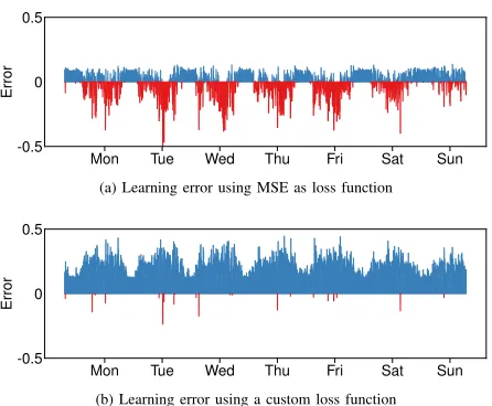
The issues above affect even current state-of-the-art Deep Learning architectures, which thus fall short of providing a complete solution to the problem of intelligent resource orchestration. For instance, the technique in [14] predicts future demands so as to minimize an absolute error, hence deviating as little as possible from the real demand. As shown in Fig. 1a, this risks to cause substantial underprovisioning, with a high cost for the operator in terms of subscribers’ churn rates, as well as of significant fees for violating Service-Level Agreements (SLAs) with tenants. The plot makes it
Mon Tue Wed Thu Fri Sat Sun -0.5
0 0.5
Error
(a) Learning error using MSE as loss function
Mon Tue Wed Thu Fri Sat Sun -0.5
0 0.5
Error
(b) Learning error using a custom loss function
Fig. 1: Prediction error in (a) traffic and (b) capacity forecast.
clear that, if mobile network operators allocate resources based on a plain traffic predictor, SLA violations will occur all the time. A strategy of blind, fixed overprovisioning on top of the demand forecast is also a highly inefficient workaround. Constantly allocating a static (and arbitrarily set) amount of resources above those estimated may be acceptable in the current 4G monolithic architecture, but will become extremely expensive when repeated across the high number of network slices expected to characterize next-generation systems [15].
In the light of these considerations, we believe thatcapacity
forecasting is a problem that has to be tacked as a whole.
By predicting capacity rather than demand, we (i) directly
obtain the complete information needed by the orchestrators
(i.e., the capacity to be allocated), and (ii) can explicitly
include all considerations on overdimensioning, SLA, and related economic costs in the problem formulation.
In this paper, we propose Deep Learning algorithms de-signed to natively take into account the specific requirements of capacity forecasting, and automatically drive the anticipa-tory resource allocation. The ultimate goal of such learning algorithms is to provide a resource allocation forecast like the one depicted in Fig. 1b: the demand is always anticipated with the minimum amount of overprovisioning that reduces the risk of SLA violations.
III. LEARNING FOR COST-AWARE ORCHESTRATION
Owing to the complexity of the resource orchestration task, and the availability of large amounts of historical training data, Deep Learning is a prime candidate to implement intelligence in mobile networks [16]. Deep Learning architectures are employed for multiple purposes: classification, where the output is the probability that a given input belongs to a specific category; forecasting, where the objective is to predict the next sample of a function given knowledge of the past; reinforcement, where the goal is to derive the optimal policy to maximize (resp., minimize) some revenue (resp., cost).
is composed by an input layer that takes a portion of the past mobile traffic time series, one or more hidden layers that extract its relevant features for prediction, and an output layer made by a single linear neuron that provides the forecast for the next orchestration time slot. In our analysis, we consider
only fully connected layers (i.e., layers where each neuron
is connected with all the neurons of the successive layer), due to their mathematical tractability; however, the approach
can be extended to any type of layer (e.g., Convolutional,
Pooling, etc.). Also, the architecture always terminates with an output layer applying a linear function since the expected output could assume any value.
A. Loss functions: a primer
The loss function is a key element in a Deep Learning architecture. In a nutshell, the loss function measures the error between the output estimation of the Deep Learning architecture and the real sample. The current error value is then back-propagated through the network layers in order to minimize future errors. Specifically, back-propagation is performed by evaluating the contribution of each weight and bias to the error, and updating them in the direction that minimizes the loss. As such a notion of direction is derived by the partial derivatives of the error with respect to the weights and biases, the loss function needs to be differentiable.
It is important that the loss function is chosen appropriately, based on the nature of the problem to be solved. For instance, in classification problems where the output is represented as the probability that a certain input belongs to a particular category, loss functions based on probability estimates, like cross-entropy, are utilized. In regression or forecasting tasks, loss functions based on linear output, like Mean Squared Error (MSE) or Mean Absolute Error (MAE), are most suitable since the output of the network can assume a continue value range. Therefore, loss functions based on linear output are espe-cially suitable also for capacity forecasting, where the output is similarly a continue variable. As mentioned above, MSE and MAE are two of the popular functions utilized in regression
problems (although others are found in the literature, e.g.,
Smooth MAE), yet they are not adequate for capacity
fore-casting. The reason is that they treat in the same waynegative
(i.e., SLA violations) andpositive(i.e., capacity excess) errors.
To address this issue, in the following we design a new, dedicated loss function based on linear output and tailored to capacity forecasting, thanks to its capability to differentiate SLA violations from overprovisioning.
B. α-OMC: a loss function for capacity forecast
As discussed in Section II, the monetary cost incurred by a network operator while running a network slice on its
infrastructure is due to two main components: (i) the cost
of overprovisioningthe network with more resources than the
ones actually needed, and (ii) the cost due to SLA violations,
that are monetary compensation paid by the network operator to its tenants in case of unserviced traffic.
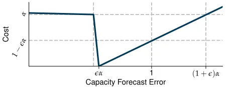
0
Capacity Forecast Error
Cost
γ
β
Fig. 2: Generic loss function for network resource
orchestra-tion:f(x)are in red, forx <≤0,g(x)are in blue, forx≥0.
eα 1 (1+e)α
Capacity Forecast Error 1−
eα α
Cost
Fig. 3: Actualα-OMC loss function. Asis a very small value,
the function is close toxin the overprovisioning domain.
These two components need to be modeled in different ways according to the desired point of operation of the system. As mentioned in Section III-A, the loss function steers the behaviour of the neural network by adjusting the weights of the neurons according to the error between the estimated value and the real one. Thus, a custom loss function for the capacity
forecasting problem is composed by a term f(x) that deal
with the resource overprovisioning costs, and a term g(x)
that models the cost for the resource violation penalties. The
variable x represents the discrepancy between the real and
estimated values at each orchestration interval.
The shape of overall cost functionf(x) +g(x)is depicted
in Fig. 2. A perfect algorithm (i.e., anoracle) always keeps the
system in the perfect operation point x∗= 0, so in this point
no penalty is introduced,i.e.,f(x∗) =g(x∗) = 0. Of course,
it is very unlikely that the prediction always matches the real demand, so a penalty value is back-propagated depending on
whetherxis above or below the target operation pointx∗.
1) g(x), a reactive approach to SLA violations: When the orchestrated resources are less than those needed in reality (i.e., x < x∗) the tenant receives a monetary compensation from the network operator. This is the case of, for instance, an SLA that guarantees a proportional compensation depending on the number of time intervals in which an operator fails to
meet the requirements set by a tenant (e.g., the total bandwidth
of its users). Thus, the system has to learn that the operation
point x∗ is actually higher than the currently estimated one
through a penaltyβ, which is applied as soon as the estimation
falls below the real value. The parameterβ can be customized
depending on the scenario: higher values may be used for cases
in which reliability is paramount (e.g., an URLLC network
slice), while lower values can be applied where KPIs are
bring the system toward x > x∗, incurring hence in higher deployment costs, as discussed next.
2) f(x), a monotonically increasing cost for resource over-provisioning: While SLA violations depend on the agreements between the tenants and the operator, the over-provision cost solely depends on the network operator, and more specifically on its OPEX in allocating excess capacity. We assume that such a cost grows with the additional unused capacity, and
model it as a monotonically increasing function of x that is
only applied whenx > x∗. The exact expression off(x)may
vary, and be, e.g., linear (i.e., f(x) = γx), super-linear (i.e.,
f(x) =xγ), or exponential (i.e., f(x) =eγx). In our study,
we will consider a linear function, as portrayed in Fig. 2.
The parameterγis configurable by the operator, and
repre-sents the monetary cost of resource allocation: for instance,
resources at the edge (i.e., spectrum) are typically scarcer
and more expensive to deploy than those in a network core
datacenter. Therefore, a positive error xin case of expensive
(i.e., high-γ) resources will tend to bring the system to a lower
estimation, with higher risks to hit the SLA violation zone.
3) Balancing the two cost contributions: In general,β and
γ are highly intertwined: β can be seen as the maximum
amount of resources a network operator is willing to add instead of incurring an SLA violation, which is in turn a
function of γ. Therefore, in the following, we express the
custom loss as a function of α= β
γ.
As explained in Section III-A, the loss function shall be differentiable in all its domain. This forces us to introduce
minimum slopes of intensity(a very small value) forx <0
and at x= 0. We name the resulting loss function Operator
Monetary Cost, which has a single configurable parameter α.
The final expression ofα-OMC is:
α-OMC(x) =
α−·x if x≤0
α−1
x if 0< x≤α
x−α if x > α.
(1)
Fig. 3 provides a sample illustration of (1) above.
IV. CONVERGENCE ANALYSIS OFα-OMC
Given the α-OMC loss function defined in Sec. III-B we
study its theoretical properties. Specifically, we are interested in showing that it is a suitable function to be employed in neural network architectures, and that is compatible with backpropagation algorithms.
Let us write theα-OMC loss function for a given epoch as:
L(x) = 1
N
N X i=1
(l1(x) +l2(x) +l3(x)),
l1(x) =−x+α, wherex≤0
l2(x) =− 1
x+α, where0≤x≤α
l3(x) =x−α, wherex≥α.
Here,xis the difference betweeno=hw,hi+bandy, which
represent the prediction and the real output, respectively. Also,
error contributions are summed overNbatchesiin the epoch.
The partial derivative of the loss function with respect to
the output of the final layerois then:
∂L ∂o =
1
N
N X i=1
∂l1(x)
∂o + ∂l2(x)
∂o + ∂l3(x)
∂o
where,
∂l1(x)
∂o =−, wherex≤0,
∂l2(x)
∂o =−
1
, where0≤x≤α,
∂l3(x)
∂o = 1, wherex≥α.
As we can see, (i) the obtained partial derivative are
monotonic, (ii) they do not vanish if the error is very high,
and (iii) they form a piece-wise linear (and, more precisely,
constant) function.
The monotonicity together with the no-vanish property
ensure that α-OMC leads to convergence, since the partial
derivatives always lead to the minimums’ direction and main-tain a non-zero value that avoids getting stuck in case the of a too high initial error [17]. Furthermore, the resulting partial derivatives are not only piece-wise linear but also constant: according to [17], the convergence speed under this circumstances is faster, especially when using first order optimization methods such as the well-known Adam [18].
Although it may be possible to design different classes of loss functions that present the characteristics defined in
Section III-B,α-OMC already provides desirable convergence
properties that make it very suitable for the capacity forecast-ing problem, as discussed in the next section.
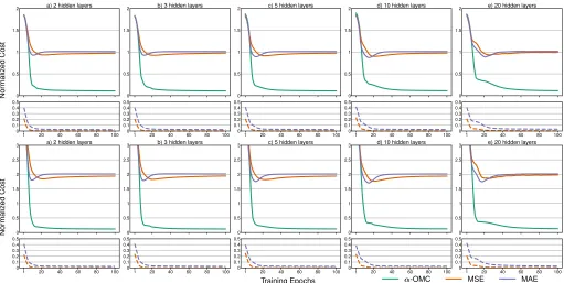
V. EMPIRICAL EVALUATION OFα-OMC
In order to evaluate the effectiveness of the proposed
loss function, we compare α-OMC against two classic loss
functions employed in forecasting problems: MSE and MAE. Experiments are carried out under different neural network configurations. Specifically, we use five different architectures, each composed by fully connected layers with a variable number of hidden layers that ranges from 2 to 20. Each hidden layer consists of 16 neurons followed by a ReLU activation function, and the whole model is trained using Adam [18] with
a learning rate of 10-4 during 100 epochs.
We leverage real-world measurement data that describes the traffic generated by the YouTube video streaming service in a mobile network deployed in a large metropolitan region in Europe. We assume that such traffic is serviced at a single datacenter, where the operator needs to anticipate the resources
(e.g., CPU time and memory for virtual machines) required to
accommodate the service demand. The orchestration occurs over 5-minute intervals, which is reasonable in network in-frastructures supporting NFV [19], and for standard Virtual Infrastructure Managers [20].
0 0.5 1 1.5
2 a) 2 hidden layers
0 0.5 1 1.5
2 b) 3 hidden layers
0 0.5 1 1.5
2 c) 5 hidden layers
0 0.5 1 1.5
2 d) 10 hidden layers
0 0.5 1 1.5
2 e) 20 hidden layers
1 20 40 60 80 100
0 0.1 0.2 0.3 0.4 0.5
1 20 40 60 80 100
0 0.1 0.2 0.3 0.4 0.5
1 20 40 60 80 100
0 0.1 0.2 0.3 0.4 0.5
1 20 40 60 80 100
0 0.1 0.2 0.3 0.4 0.5
1 20 40 60 80 100
0 0.1 0.2 0.3 0.4 0.5 Training Epochs Nor maliz ed Cost
2-OMC MSE MAE
0 0.5 1 1.5 2 2.5
3 a) 2 hidden layers
0 0.5 1 1.5 2 2.5
3 b) 3 hidden layers
0 0.5 1 1.5 2 2.5
3 c) 5 hidden layers
0 0.5 1 1.5 2 2.5
3 d) 10 hidden layers
0 0.5 1 1.5 2 2.5
3 e) 20 hidden layers
1 20 40 60 80 100
0 0.1 0.2 0.3 0.4 0.5
1 20 40 60 80 100
0 0.1 0.2 0.3 0.4 0.5
1 20 40 60 80 100
0 0.1 0.2 0.3 0.4 0.5
1 20 40 60 80 100
0 0.1 0.2 0.3 0.4 0.5
1 20 40 60 80 100
0 0.1 0.2 0.3 0.4 0.5 Training Epochs Nor maliz ed Cost
α-OMC MSE MAE
Fig. 4: Average operator’s economic cost versus the learning epochs, under α-OMC, MSE and MAE loss functions. Smaller
plots at bottom show the actual errors minimized by MSE and MAE. Top: α= 2. Bottom:α= 4.
the last 30 minutes of traffic as input1. In line with our
discussion of economic costs induced by overprovisioning and underprovisioning, the overall monetary penalty incurred by a network operator is computed as the number of time steps with
SLA violations multiplied by a factor α, plus the amount of
excess predicted capacity2. To ease the interpretation of results,
the monetary penalty is then transformed into a normalized cost, dividing it by the instantaneous expenditure peak.
A. Cost minimization capability
We start by evaluating the dynamics of the learning algo-rithm, testing the behaviour of each loss function over time. Specifically, we measure the normalized cost when using the different loss functions and architectures.
The top row of Fig. 4 shows how the test average normalized cost o network operation vary during the training phase for
5 different architectures, under α = 2. While the 2-OMC
loss function minimizes the operator’s cost, both MAE and
MSE converge to a fixed fee that depends on the value of α.
Indeed, when doublingαfrom a value of 2 to a value of 4, as
showed in the bottom row of Fig. 4, also the fee doubles to a value of 2. This confirms that classical loss functions are not effective when dealing with capacity forecasting, resulting in high penalties for operators.
The smaller plots below each row in Fig. 4 depict the
average normalized loss,i.e.,, a metric that does not consider
monetary factors, but purely measures the distance of the
1We experimented with longer history input, without noticeable differences.
2We remark that multiplying the number of violations by α returns a
dimensionally correct penalty, whose unit can be interpreted as the cost of allocating resources to service one additional byte of traffic.
prediction to the actual traffic demand. These curves illustrate that both MAE and MSE do minimize the overall discrepancy from the target signal, which, however, is not aligned with the
actual monetary cost. Conversely,α-OMC steers the
forecast-ing capability of the Deep Learnforecast-ing architecture by weightforecast-ing the different sources of cost: it goes beyond legacy traffic demand estimation, and performs an actual capacity forecast.
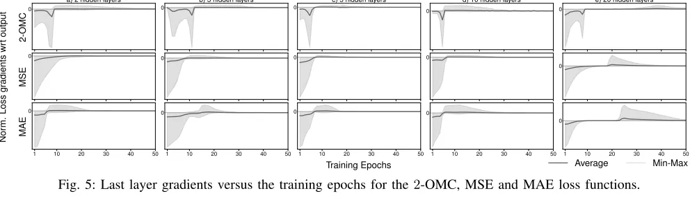
B. Gradient behavior
Backpropragation algorithms work by updating the weights and biases of each layer proportionally to the value of the gradient of the loss function. Thus, a relevant aspect to
investigate is how the 2-OMC loss gradients behave with
respect to the weights and biases of the last layer.
In Fig. 5 we show the maximum, minimum and mean
value of all gradients (i.e., weights and biases) of a 2-OMC
loss function with respect to the last layer. We observe that, after fluctuations due to the initial randomness, all gradients converge to 0. This means that the last-layer weights and biases do not contribute anymore to the prediction error as they reached a minimum point in the loss function (which could be global or local). Fig. 5 also give us an estimation of the convergence speed: after around 50 epochs all gradients converge under any neural network architecture.
C. Forecast comparison
As last experiment, we compare the forecasting obtained on the test dataset after training our neural network with 20
hidden layers employing the 2-OMC, MSE and MAE loss
0
a) 2 hidden layers
0
b) 3 hidden layers
0 c) 5 hidden layers 0 d) 10 hidden layers 0
e) 20 hidden layers
0 0 0 0
0
1 10 20 30 40 50
0
1 10 20 30 40 50
0
1 10 20 30 40 50
0
1 10 20 30 40 50
0
1 10 20 30 40 50
0
Training Epochs
Nor
m.
Loss
gr
adients
wr
toutput 2-OMC
MSE
MAE
Average Min-Max
Fig. 5: Last layer gradients versus the training epochs for the2-OMC, MSE and MAE loss functions.
0 0.5 1
Nor
maliz
ed
traffic
Service demand Capacity forecast
Mon Tue Wed Thu Fri Sat Sun
-0.5 0 0.5
Error
(a) 2-OMC
0 0.5 1
Nor
maliz
ed
traffic
Service demand Capacity forecast
Mon Tue Wed Thu Fri Sat Sun
-0.5 0 0.5
Error
(b) MSE
0 0.5 1
Nor
maliz
ed
traffic
Service demand Capacity forecast
Mon Tue Wed Thu Fri Sat Sun
-0.5 0 0.5
Error
(c) MAE
Fig. 6: Capacity forecasting with a 20-hidden-layer architecture for the 2-OMC, MSE and MAE loss functions. Top: actual
and predicted time series. Bottom: overprovisioning (blue) and underprovisioning (red) errors. Figure best viewed in colors.
in Fig. 6a–6c, confirm that (i) the deployed neural network
architecture is able to provide an accurate forecast for all of
the different loss functions, and (ii) only a cost-aware loss
function like 2-OMC is able to minimize the actual network
operation penalty, almost completely avoiding expensive SLA-violations, and minimizing the overprovisioning in doing so. State-of-the-art loss functions such as MSE and MAE do not distinguish between negative and positive errors, and induce an unacceptable high number of SLA violations.
VI. CONCLUSIONS
In this paper we made the case for capacity forecasting in mobile network resource orchestration. We discussed how this original problem can be solved by Deep Learning algorithms with custom loss functions that consider real network
opera-tional costs. We proposed α-OMC, the very first cost-aware
loss function for network resource orchestration, and assessed its convergence properties both theoretically and empirically.
Our results show the effectiveness ofα-OMC in meeting real
network requirements when compared to legacy, state-of-the-art loss functions for traffic demand prediction.
ACKNOWLEDGMENT
The work of University Carlos III of Madrid was supported by the H2020 5G-MoNArch project (Grant Agreement No. 761445) and the work of NEC Europe Ltd. by the 5G-Transformer project (Grant Agreement No. 761536).
REFERENCES
[1] P. Hedman, “NGMN 5G P1 Requirements & Architecture Work Stream End-to-End Architecture – Description of Network Slicing Concept,”
NGMN Alliance White Paper, 2016.
[2] ETSI, “Network Function Virtualization (NFV) Management and Or-chestration,”NFV-MAN 001 v1.1.1, 2014.
[3] ETSI, “Improved operator experience through Experiential Networked Intelligence (ENI),”ETSI White Paper No.22, 2017.
[4] EC H2020 5G Infrastructure PPP (5G-PPP), “Pre-structuring Model, version 2.0,”5G-PPP White Paper, 2014.
[5] M. Joshi and T. H. Hadi, “A Review of Network Traffic Analysis and Prediction Techniques,”arXiv:1507.05722 [cs.NI], 2015.
[6] F. Xu,et al., “Big data driven mobile traffic understanding and forecast-ing: A time series approach,”IEEE Trans. Serv. Comput., 9(5), 2016. [7] M. Zhanget al., “Understanding urban dynamics from massive mobile
traffic data,”IEEE Trans. Big Data, 2017.
[8] S. T. Au, G.-Q. Ma, and S.-N. Yeung, “Automatic forecasting of double seasonal time series with applications on mobility network traffic prediction,”JSM Proc., Business and Economic Statistics Section, 2011. [9] S. Ntalampiras, M. Fiore, “Forecasting mobile service demands for
anticipatory MEC,”IEEE WoWMoM, 2018.
[10] R. Liet al., “The prediction analysis of cellular radio access network traffic: From entropy theory to networking practice,”IEEE Comm. Mag., 52, 2014.
[11] M. Z. Shafiq et al., “Characterizing and modeling internet traffic
dynamics of cellular devices,”ACM SIGMETRICS, 2011.
[12] J. Wang et al., “Spatiotemporal modeling and prediction in cellular networks: A big data enabled deep learning approach,”IEEE INFOCOM, 2017.
[13] A. Y. Nikraveshet al.“An experimental investigation of mobile network traffic prediction accuracy,”Int. Journal of Big Data, 3, 2017. [14] C. Zhang, and P. Patras, “Long-Term Mobile Traffic Forecasting Using
Deep Spatio-Temporal Neural Networks,”ACM MobiHoc, 2018.
[15] C. Marquez, M. Gramaglia, M. Fiore, A. Banchs and X. Costa-Perez, “How should I slice my network? A Multi-Service Empirical Evaluation
of Resource Sharing Efficiency,”ACM MobiCom, 2018.
[16] C. Zhang, P. Patras, and H. Haddadi, “Deep learning in mobile and wireless networking: A survey,”arXiv:1803.04311 [cs.NI], 2018 [17] K. Janocha and W. M. Czarnecki, “On loss functions for deep neural
networks in classification”arXiv:1702.05659 [cs.LG], 2017.
[18] D. P. Kingma and J. Ba, “Adam: A method for stochastic optimization,”
arXiv:1412.6980 [cs.LG], 2014.
[19] F. Z. Yousaf and T. Taleb, “Fine-grained resource-aware virtual network function management for 5G carrier cloud,”IEEE Network, 30(2), 2016. [20] J. G. Herrera and J. F. Botero, “Resource allocation in NFV: A