Hybrid Machine Learning Model of Support Vector Machine and Fruit Fly Optimization Algorithm for Prediction of Remaining Service Life of Flexible Pavement

Article

1

Hybrid Machine Learning Model of Support Vector

2

Machine and Fruit Fly Optimization Algorithm for

3

Prediction of Remaining Service Life of Flexible

4

Pavement

5

Nader Karballaeezadeh 1, Adrienn Dineva 2, Amir Mosavi 3, Narjes Nabipour 4,*, Shahaboddin

6

Shamshirband 5,6,_{*, Danial Mohammadzadeh} 7,8

7

1_{Department of Civil Engineering, Shahrood University of Technology, Shahrood, Iran:}

8

[email protected]

9

2 _{Kalman Kando Faculty of Electrical Engineering, Obuda University, 1034 Budapest, Hungary}

10

3 _{Queensland University of Technology (QUT), 130 Victoria Park Road, Queensland 4059, Australia}

11

4 _{Faculty of Information Technology, Ton Duc Thang University, Ho Chi Minh City, Vietnam;}

12

5 _{Department for Management of Science and Technology Development, Ton Duc Thang University, Ho Chi}

13

Minh City, Vietnam

14

6 _{Faculty of Information Technology, Ton Duc Thang University, Ho Chi Minh City, Vietnam}

15

7 _{Department of Civil Engineering, Ferdowsi University of Mashhad, Mashhad 9177948974, Iran}

16

8 _{Department of Elite Relations with Industries, Khorasan Construction Engineering Organization, Mashhad}

17

9185816744, Iran

18

* Correspondence: [email protected]

19

20

Abstract: Remaining service life (RSL) of pavement, as a sign of future pavement performance, has

21

always received growing attention from pavement engineers. The RSL describes the time from the

22

moment of pavement inspection until such a time when a major repair or reconstruction is required.

23

The conventional approach to determining RSL involves using non-destructive tests. These tests, in

24

addition to being costly, interfere with traffic flow and compromise users' safety. In this paper,

25

surface distresses of pavement have been used to estimate the pavement’s RSL in order to eliminate

26

the aforementioned problems and challenges. To implement the proposed theory, 105 flexible

27

pavement segments were taken from Shahrood-Damghan Highway (Highway 44) in Iran. For each

28

pavement segment, the type, severity, and extent of surface damage and pavement condition index

29

(PCI) were determined. The pavement RSL was then estimated using non-destructive tests include

30

Falling Weight Deflectometer (FWD) and Ground Penetrating Radar (GPR). After completing the

31

dataset, the modeling was conducted to predict RSL using three techniques include Support Vector

32

Regression (SVR), Support Vector Regression Optimized by Fruit Fly Optimization Algorithm

33

(SVR-FOA), and Gene Expression Programming (GEP). All three techniques estimated the RSL of

34

the pavement by selecting the PCI as input. The Correlation Coefficient (CC), Nash-Sutcliffe

35

efficiency (NSE), Scattered Index (SI), and Willmott’s Index of agreement (WI) criteria were used to

36

examine the performance of the three techniques adopted in this study. In the end, it was found that

37

GEP with values of 0.874, 0.598, 0.601, and 0.807 for CC, SI, NSE, and WI criteria, respectively, had

38

the highest accuracy in predicting the RSL of pavement.

39

Keywords: hybrid machine learning model; transportation infrastructure; flexible pavement;

40

remaining service life prediction; pavement condition index; support vector regression; fruit fly

41

optimization algorithm (FOA); gene expression programming (GEP); SVR-FOA

42

43

44

1. Introduction

45

Predicting future pavement conditions and estimating its service life is one of the fundamental tasks

46

of pavement engineers in pavement management systems (PMSs), as the future network conditions

47

act as a prerequisite for the planning, prioritization, and allocation of resource [1]. In general,

48

pavement management activities are split into two categories [2]: network-level management and

49

project-level management. Project-level management specifies roads that need to be repaired, repair

50

process, and repair timetable. Therefore, predicting future conditions of pavement is essential for

51

network-level management [2]. Forecasting pavement future conditions will require ongoing

52

pavement assessment and inspection that will improve the operational quality of maintenance

53

operations [3,4]. On the other hand, network-level management focuses on determining the budget

54

required to preserve the pavement network at the standard level. Hence, it is indispensable to

55

determine the remaining service life (RSL) of payment at this level of management [2]. Various factors

56

such as traffic, characteristics of pavement materials, subgrade properties, climatic conditions, and

57

maintenance quality have a destructive impact on the road pavement. As a result, pavement service

58

life is surrounded by uncertainties that complicate the prediction of RSL [5].

59

In recent years, several indices have been developed for pavement evaluation. One of these indicators

60

is the pavement condition index (PCI), which represents the general conditions of the pavement

61

surface and ranges from zero for a practically unusable pavement to 100 for a flawless pavement. PCI

62

is determined based on pavement inspection results in terms of type, severity, and extent of distresses

63

[6,7]. The PCI estimation requires an experienced inspector to determine PCI after a thorough

64

inspection of pavement surface distresses. Conversely, RSL of pavement, which is one of the pillars

65

of network-level pavement management, is determined by applying Falling Weight Deflectometer

66

(FWD) non-destructive test. In this test, a traffic lane is first blocked. Then an impulsive loading is

67

applied to the pavement to induce pavement surface deflections. By analyzing pavement surface

68

deflections, the RSL is calculated. A key point in calculating the RSL using the above method is

69

knowing the pavement layers thickness for the analysis of deflections. The thickness of the pavement

70

layers is determined by the Ground Penetrating Radar (GPR) non-destructive test. As a result, two

71

non-destructive tests are required to determine the RSL of pavement. Also, traffic interference during

72

FWD and GPR tests should not be forgotten[8].

73

In light of the above, the current method of determining RSL is not only costly but also compromises

74

the safety of inspectors due to traffic interference during testing. Given the limited budget resources

75

of transportation agencies, determining the RSL of pavement to manage a pavement network

76

represents one of the ongoing concerns of such companies[4]. One way to overcome these problems

77

is to employ artificial intelligence models. In this paper, three methods of Support Vector Regression

78

(SVR), SVR-FOA (Support Vector Regression Optimized by Fruit Fly Optimization Algorithm), and

79

Gene Expression Programming (GEP) have been applied to predict the RSL of road pavements. For

80

PCI is an index adopted in the project-level pavement management process. Hence, this index is

82

specified before entering network-level pavement management. As such, using PCI for network-level

83

management operations, such as estimation of RSL, will contribute to the overlapping of activities

84

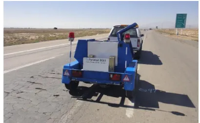
and saving time. The methods presented in this paper, by excluding non-destructive tests from the

85

process of determining the RSL of pavement, drastically reduce costs associated with the pavement

86

network management. On the other hand, by eliminating non-destructive tests, traffic interference

87

during testing and the potential safety hazards to inspectors are also eliminated. The data required

88

for developing the methods proposed in this paper was collected from Shahrood-Damghan highway

89

in Semnan province, Iran. The pavement type of this highway is flexible. In this highway, a 100-m

90

long pavement segment was taken from the beginning of each kilometer, and after assessing the

91

surface distresses of each segment, its PCI was calculated. In the next step, FWD and GPR tests were

92

applied to the selected segments to determine the RSL. Finally, using three SVR, SVR-FOA and GEP

93

methods, the RSL modeling based on PCI was implemented.

94

This paper is organized as follows: Section 2 offers a review of studies on the prediction of RSL.

95

Section 3 introduces the method employed in this study. This section is made of four sub-sections

96

titled PCI, RSL, artificial intelligence techniques, and case study. In Section 4, the results of the

97

analyses are presented and discussed. Finally, the conclusions are drawn in Section 5.

98

99

2. Literature Review

100

PMS is an assessment management system (AMS) used by road network administrators to maintain

101

the entire network at the desired level. Predicting pavement performance is a key factor in PMSs [9].

102

The models of predicting pavement’s RSL fall in the category of the pavement performance

103

prediction models. In this section, studies carried out by other researchers on predicting RSL are

104

reviewed. Table 1 lists the results of studies that have strived to estimate RSL to date.

105

106

Table 1. Models for the prediction of RSL[10-17]

107

Category Model inputs Equation Author

1. Based on

pavement

responses

ℇt = Tensile strain at the

bottom of the asphalt layer,

E1 = Elastic modulus of

asphalt.

RSLfatigue= f1(εt)−f2(E1)−f3

Huang

(1993)

ℇc = Compressive strain at the

top of the subgrade. RSLrutting = f4(εc)

−f5 Huang

(1993)

ℇt = Tensile strain at the

asphalt layer bottom,

RSLfatigue= 0.1001(εt)

− 3.565(MR)−1.4747

Das &

Pandey

MR = Resilient modulus.

ℇr = Horizontal tensile strain

at the bottom of the asphalt

layer,

EAC = Modulus of asphalt.

ln(RSLfatigue) = a − b ln(εr)

− c ln(EAC)

Hossain &

Wu (2002)

ℇt = Tensile strain at the

asphalt layer bottom. RSLfatigue= K(εt)

−C Park & Kim

(2003)

2. Based on

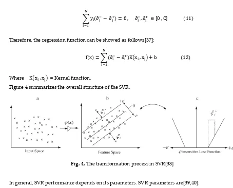
pavement

quality

indices

IRI = International roughness

index. RSL =

ln(IRIterminal

a )

b − (Current age)

Al-suleiman &

Shiyab

(2003)

PCI = Pavement Condition

Index. RSL = 4.1872 ln(PCI) − 14.728

Setyawan

et al (2015)

3. Based on

the result of

the

non-destructive

test

δ = Pavement surface

curvature,

δ = D0− D20

RSLfatigue= α (

1

0.0023δ + 0.00002)

β _Saleh

(2016)

AUPP = Area under

pavement profile,

AUPP

=5D0− 2D30− 2D60− D90

2

RSLfatigue

= α( 1

0.0000023AUPP0.912)

β

Saleh

(2016)

108

In Table 1, the models of determining RSL of pavement are divided into three categories based on the

109

model inputs:

110

• First category: Models that predict RSL based on the response (stress and strain) of pavement to

111

the applied loads.

112

• Second category: Models that predict RSL based on pavement quality indices.

113

• Third Category: Models that predict RSL based on the results of pavement non-destructive tests.

114

Among the above categories, models that predict remaining pavement service based on qualitative

115

indices appear to be more appropriate. It is because such models neither call for the analysis of

116

pavement behavior and response, as in the first category nor require non-destructive tests, like the

117

third category. Instead, they estimate the RSL of the pavement by assessing pavement and calculating

118

a qualitative index in the simplest possible way. In light of the above points, in this paper, PCI has

119

results of which are displayed in Table 1. The model presented in their study was based on data

121

collected from only 5 pavement segments in the Microsoft Excel software, which cast doubt on the

122

reliability of the model. In contrast, the methods proposed in this paper are based on the data

123

gathered from more than 100 pavement segments using artificial intelligence methods.

124

In general, PCI offers a valid index accepted by all transportation agencies around the world, and it

125

is widely used in their evaluations. Compared to the current method of estimating the RSL of

126

pavements (using two non-destructive FWD and GPR tests), the proposed method provides a far

127

simpler, safer and less costly way of estimating RSL.

128

129

3. Methodology

130

3.1. Pavement Condition Index (PCI)

131

PCI was developed by U.S. Army Crops of Engineers as a performance benchmark for PMSs[7].

132

Extensively used in roads, parking lots, and airports, PCI is recognized as a standard practice by

133

many organizations around the world, including the Federal Aviation Administration, the American

134

Public Works Association, and the U.S. Air Force[18]. PCI is a numerical index that expresses the rate

135

of pavement surface distresses. PCI exhibits structural integrity and Surface operational condition

136

but is not able to measure structural capacity[19].

137

To determine PCI in a pavement segment, the pavement surface of the segment is inspected, and

138

their surface distresses are recorded in the assessment form. The PCI of a pavement sample unit

139

depends on the type, extent, and severity of its surface damages. In the PCI calculation process, a

140

perfect and flawless pavement receives a maximum score of 100. For defective pavements, the score

141

is deducted from 100 incommensurate with the type, extent, and severity of the damage[7,18,19]. In

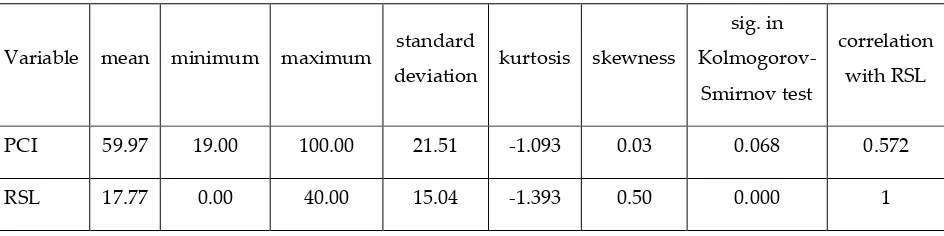
142

general, PCI can be computed using Eq. 1[4]:

143

144

PCI = 100 − ∑ni=1(Distress Score) (1)

where: PCI = Pavement Condition Index, distress Score = Score based on type, extent, and severity of

145

distresses, n = Number of distresses. The instructions for calculating distress scores are fully described

146

in ASTM D6433-07. The classification of a pavement segment based on PCI is according to Table 2.

147

148

Table 2. PCI rating scale[19]

149

Rating

Scale 0-10 10-25 25-40 40-55 55-70 70-85 85-100

Description Faile

d Serious

Very

Poor Poor Fair Satisfactory Good

150

3.2. Remaining Service Life (RSL)

The RSL of pavement under operation is a key factor in implementing PMSs. It is because learning

152

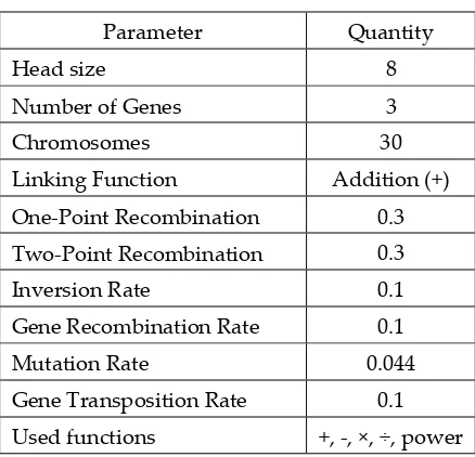
about the future conditions of the pavement network is essential for decision making, life cycle cost

153

analysis, planning and budget allocation[8,20]. In general, the definitions of RSL by different agencies

154

and departments of transportation can be split into two general categories[21]:

155

• The remaining time to reach a level of distress when the pavement needs to be rehabilitated or

156

reconstructed. For example, the Minnesota Department of Transportation (MnDOT) defines

157

the RSL as the time until the next major rehabilitation.

158

• The time until pavement conditions reach a specific condition index limit. For example, the

159

Michigan Department of Transportation (MDOT) defines the RSL based on the Michigan

160

Ride Quality Index, assuming an RSL of zero when the said index is 50.

161

The RSL of pavement segments in this paper has been determined using Heavy Falling Weight

162

Deflectometer (HWD). The HWD is an FWD, the application of which is not constricted to the road

163

and could be used for airport pavement assessment. Figure 1 shows the HWD device employed in

164

this study.

165

166

Fig. 1. HWD used in this study for determining RSL

167

168

The HWD applies a tension similar to the standard axle load (8.2 tons) to the pavement surface over

169

10 to 35 milliseconds. A number of geophones are placed on the pavement surface at specified

170

distances from the loading center. The task of the geophones is to record the pavement deflections

171

induced by the load applied with the HWD device. Standard axle load simulation in HWD is

172

generated by a series of weight drops on a loading plate placed on the pavement surface[8]. Table 3

173

reveals the details of the HWD test undertaken in this study.

174

176

Table 3. HWD test details[22]

177

Parameter Value

Tension (Kpa) 600 – 900

Number of geophones 9

Geophone distance from center of laoding plate

(cm)

0, 20, 30, 45, 60, 90, 120, 150, and

180

Number of weights falling Four times

Loading plate radius (mm) 150

178

The deflections recorded by geophones are transferred to the central computer in HWD. In this

179

computer, the analysis of pavement surface deflections is performed using ELMOD6 software. One

180

output of this analysis is the estimation of pavement remaining service life under test.

181

A prerequisite of estimating RSL in accordance with the process described in this section is knowing

182

the thickness of pavement layers. For determining the pavement layer's thickness,

ground-183

penetrating radar (GPR) non-destructive testing was carried out for all pavement segments. GPR is

184

capable of calculating pavement thickness as a continuous profile by transmitting electromagnetic

185

waves through a transmit antenna and receiving recursive signals[23]. Table 4 shows the complete

186

details of the GPR experiment carried out in this study.

187

188

Table 4. GPR test details[24,25]

189

Parameter Value

Antenna type 1000 MHz

Record speed (km/hr) 10

Number of scanning (per meter) 10

Maximum pulse penetrating depth

(ns)

32

190

3.3. Artificial intelligent techniques

191

In this paper, the main objective is to present a new approach for predicting the RSL of flexible

192

pavements based on PCI using artificial intelligence techniques. To do so, a dataset of 105 pavement

193

segments was collected from Shahrood-Damghan highway in Iran. The data set consisted of the RSL

194

methods. GEP is an evolutionary algorithm that investigates the relationship between input and

196

output variables by developing computer programs[26]. Different from both the Genetic Algorithm

197

(GA) and Genetic Programming (GP), GEP is a combination of both introduced by Ferreira in 2001[27].

198

SVR is a supervised machine learning technique employed to solve regression problems. SVR is

199

especially popular due to its desirable management and performance in handling nonlinear

200

issues[28]. The success of an SVR in problem-solving depends on the values of its basic parameters.

201

The SVR basic parameters include C, ε, and kernel function parameters[8]. Improper values of the

202

basic parameters in the SVR can lead to under-fitting or over-fitting. Thus, optimum values must be

203

selected for these parameters during training[29]. FOA is an intelligent swarm algorithm introduced

204

by Pan in 2012, which utilizes the food searching strategy of a fruit fly to find the optimal values for

205

SVR basic parameters[30]. These methods are introduced in the following subsections.

206

207

3.3.1. Gene Expression Programming (GEP)

208

GEP is a developed GP method that solves a problem by creating expression trees (ETs). In fact, GEP

209

is an evolutionary algorithm for creating computer programs. The designed computer programs have

210

sophisticated tree structures that are trained similar to a living organism by changing size, shape, and

211

composition, and adapted to the conditions. Like living organisms, GEP programs are coded as

212

simple fixed-length linear chromosomes. Hence, GEP is a genotype-phenotype system that employs

213

a simple genome to store and transmit genetic information and adopts a complex phenotype to

214

explore and adapt to the environment. The genome consists of a chromosome or a fixed-length string

215

that combines one or more genes of the same size. In fact, each chromosome contains one or more

216

genes known as Sub-ETs. In GEP, all Sub-TEs are linked through the root with connection functions.

217

The connection functions in GEP include division, multiplication, subtraction, and addition[31].

218

Figure 2 shows an instance of the genotype-phenotype structure in GEP.

219

220

221

Fig. 2. A sample of the genotype-phenotype structure in GEP[32]

222

These genes, despite their fixed length, are coded for ETs of varying size and shape. It implies that

224

the size of the coding region varies from one gene to another to allow for progressive adaptation and

225

evolution. Each gene has a coding area called Open Reading Frame (ORF), which after being coded

226

as an expression tree, provides a solution to the problem[33]. Figure 3 demonstrates the coding region

227

(ORF), non-coding region, and the expression tree for a gene.

228

229

230

Fig. 3. The coding region (ORF), no-coding region, and expression tree in a gene [34]

231

Like other evolutionary approaches, GEP begins by randomly generating initial population

232

chromosomes. In the first population, each chromosome is assessed based on the fitness function and

233

receives a fitness value. Various fitness functions have been used in GEP, including Root Relative

234

Squared Error (RRSE), Relative Square Error (RSE), Root Mean Square Error (RMSE), and Mean

235

Square Error (MSE)[26]. The proper chromosomes are more likely to be picked in the next generation.

236

After being selected, chromosomes are amended by genetic operators (including transposition,

237

inversion, mutation, recombination, and gene crossover) and then reconstructed. This process is

238

sustained until a suitable solution or the maximum number of generations is reached[26,35].

239

240

3.3.2. Support Vector Regression (SVR)

241

The SVR is actually a support vector machine (SVM) used for regression problems. Supervisor

242

machine learning techniques, including SVR, utilize Structural Risk Minimization (SRM), while

243

conventional neural networks use Empirical Risk Minimization (ERM). ERM minimizes the error of

244

training samples, but SRM is able to minimize a higher level of error. As a result, SVM is capable of

245

overcoming the deficiencies of conventional neural networks[8,28]. The main idea in SVR is to map

246

nonlinear information into a higher dimensional space and then solve a linear regression problem in

247

the new space[28,36,37]. In the new space, a simple linear kernel function is adopted to solve the

248

problem. However, in complex problems, a simple linear kernel function will be inadequate. The

249

k(x, z) =< φ(x). φ(z) > (2)

Each kernel function must have two features[28]:

251

1. Symmetricity

252

k(x, z) =< φ(x). φ(z) >=< φ(z). φ(x) >= k(z, x) (3)

2. Compliance with the Cauchy-Schwartz criterion

253

k(x, z)2_{=< φ(x). φ(z) >}2 _{≤ ‖φ(x)‖}2_‖φ(z)‖2 ₍₄₎

These two conditions guarantee that the new space is definable by the kernel function. The most

254

famed kernel functions are Polynomial kernel, Radial Basis Functional kernel, Linear kernel, and

255

Sigmoid kernel [37]. Given the above explanation, it is clear that SVR requires an appropriate function

256

to explain the nonlinear relationship between input (xi) and output (yi)[37]:

257

f(xi) = w. φ(xi) + b (5)

where: φ(xi) = Transformation Function, w = Weight, b = Bias. w and b are obtained by minimizing

258

the following function, which is known as the regularized risk function [37]:

259

R(w) =1

2‖w‖

2_{+ C ∑ L}

ε(yi, f(xi))

N

i=1 (6)

where:

260

1

2‖w‖

2 _{= Regularization term,}

261

C = Penalty coefficient,

262

Lε(yi, f(xi)) = ε-insensitive loss function:

263

Lε(yi, f(xi)) = max{0, |yi, f(xi)| − ε} (7)

where: ε = Permitted error threshold.

264

To solve the optimization boundaries, two factors of ξ and ξ∗ are defined[37]:

265

minf(w,ξ,ξ∗) =1

2‖w‖

2_{+ C ∑}N _{( ξ ,ξ}∗₎

i=1 (8)

Subject to:

266

{ yi− [w. φ(xi)] − b ≤ ε +ξ , ξ≥ 0

[w. φ(xi)] + b − yi≤ ε +ξ∗ , ξ∗≥ 0

(9)

We now need to define a Lagrange function based on the objective function and boundary

267

conditions[37]:

268

269

maxH(∂i−, ∂i+) = −

1

2∑ ∑(∂i

−_{− ∂} i +_)(∂

j −_{− ∂}

j +_)K(x

i , xj) N

j=1 N

i=1

+ ∑ yi(∂i−− ∂i+)

N

i=1

− ε ∑ yi(∂i−+ ∂i+)

N

i=1

(10)

∑ yi(∂i−− ∂i+) N

i=1

= 0 , ∂i−, ∂i+ ∈ [0 , C] (11)

Therefore, the regression function can be showed as follows[37]:

271

f(x) = ∑(∂i−− ∂i+)K(xi , xj)

N

i=1

+ b (12)

Where K(xi , xj) = Kernel function.

272

Figure 4 summarizes the overall structure of the SVR.

273

274

Fig. 4. The transformation process in SVR[38]

275

276

In general, SVR performance depends on its parameters. SVR parameters are[39,40]:

277

• ε: this parameter supervises the width of the ε-insensitive zone, used to fit the training data.

278

The value



279

For the bigger ε, estimates are more ‘flat’, and the fewer support vectors are chosen.

280

• C: this parameter specifies the trade-off between the complexity of the model and the grade

281

to which deviations larger than ε are bearable in optimization formulation.

282

• 𝛾: this parameter determines the relation between error minimization and smoothness of the

283

estimated function.

284

These parameters are chosen by the user based on prior knowledge of SVR, so this method is not

285

suitable for non-professional users. Various algorithms have been developed to optimize the amounts

286

of SVR parameters. In the following subsection, one of the optimization algorithms used in this paper

287

is introduced.

288

289

3.3.3. Fruit Fly Optimization Algorithm (FOA)

290

FOA is an optimization algorithm developed based on the food search behavior of the Drosophila

291

insect[30]. The fruit fly has superior smell and vision senses, which discriminates it from other insects.

292

Fruit flies track the smell of the food sources dispersed through the air and heads towards it. This

293

insect is even capable of smell tracking from a distance of 40 km. When approaching the food source,

294

shared among the fruit flies and finally, the route leading to the food source is identified[41]. Figure

296

5 illustrates the process of food search by a fruit fly.

297

298

Fig. 5. Food finding the iterative process of a fruit fly swarm[42].

299

300

In this paper, this optimization algorithm has been selected to find the optimal values of SVR

301

parameters, which is known as SVR-FOA. The general steps of SVR-FOA can be summarized as

302

follows[43,44]:

303

Step 1. SVR parameters (ε , C) initialization and kernel function determination

304

Step 2. Parameter initialization

305

Including the maximum number of iterations, location of initial population (X-axis, Y-axis),

306

population size, and random flight distance domain:

307

X_axis = rands(1,2) (13)

Y_axis = rands(1,2) (14)

Step 3. Population initialization

308

A random location (Xi, Yi) and food founding distance are assigned to each fruit fly:

309

Xi = X_axis + Random value (15)

Yi = Y_axis + +Random value (16)

where: i = Population size.

310

Step 4. Population evaluation

311

The distance from origin to the food source (D) and the smell concentration parameter (S) are

312

calculated:

313

Di= √Xi2+ Yi2 (17)

Si=

1

Di (18)

S value is substituted with the fitness function or smell concentration judgment function so that the

315

smell concentration for each fruit fly location can be attained:

316

Smelli = Function (Si) (19)

Step 6. Detect the maximal smell concentration

317

At this point, the fruit fly with the highest Si is identified and located within the population.

318

319

[bestSmellbestIndex] = max (Smell) (20)

Step 7. Keep smell concentration

320

The coordinates of the maximum smell concentration are set, and the fruit fly swarm flows in that

321

direction.

322

X_axis = X(bestIndex) (21)

Y_axis = Y(bestIndex) (22)

Step 8. Iterative optimization

323

Steps 3 to 6 are repeated until the smell concentration does not show any improvement compared to

324

the previous one or the maximum number of repetitions in Step 2 is reached.

325

Step 9. Output the optimum parameter of SVR

326

327

3.4. Case study

328

To implement the theory proposed in this paper, a stretch of 105 km from Shahrood-Damghan

329

highway in Iran was selected and inspected. Given that this highway is part of the route between

330

Tehran (the capital of Iran) and Mashhad (the second most important city of Iran), it constitutes one

331

of the major roads. The highway consists of two lanes in each direction and uses the flexible pavement.

332

A prerequisite of implementing the proposed theory is to select a number of sample segments from

333

his highway. To do so, segments 100 m in length and 7 m in width were selected from the beginning

334

of each kilometer. By inspecting the selected segments, the surface distress data (type, severity, and

335

extent) of each segment was recorded in the assessment forms. The PCI of each segment was

336

calculated as described in Section 3.1. With PCI known, the RSL of the pavement segments need to

337

be known. Hence, HWD and GPR tests were performed on all segments and the average RSL of each

338

segment was determined. Figure 6 shows the position of the Shahrood-Damghan Highway as well

339

341

Fig. 6. Highway No. 44 (Shahrood-Damghan) map used in this study.

342

343

4. Results and discussion

344

The results of the analysis are presented in this subsection. First, the statistical specifications of the

345

input and output modeling variables are listed in Table 5. The data was extracted from IBM SPSS 23

346

software.

347

Table 5. Statistical characteristics of the utilized data.

348

Variable mean minimum maximum standard

deviation kurtosis skewness

sig. in

Kolmogorov-Smirnov test

correlation

with RSL

PCI 59.97 19.00 100.00 21.51 -1.093 0.03 0.068 0.572

RSL 17.77 0.00 40.00 15.04 -1.393 0.50 0.000 1

349

As depicted in Table 5, the mean PCI of all pavement segments is 59.97, which according to Table 2,

350

is indicative of the fair state of all segments. Also, the mean RSL of pavement is 17.77 years. For

351

interpreting the mean RSL, it is worth noting that ELMOD6 software does not suggest the application

352

of an overlay layer for this RSL. Hence, the average RSL of the segments is fairly desirable. Before

353

calculating the correlation coefficient of the modeling input and output, the normality of the data

354

must be determined. This is determined by kurtosis and skewness coefficients, as well as the results

355

of the Kolmogorov-Smirnov test. According to Table 5, since PCI variables have normal distribution

356

but RSL distribution is abnormal, the Spearman correlation test must be used. The correlation

357

As noted in subsection 3.3.2, SVR consists of three basic parameters (C, ε and γ), with the quality of

359

SVR performance depending on the values selected for these three parameters. Table 6 shows the

360

values of these basic parameters for the SVR as well as the optimized values of these parameters by

361

the FOA algorithm.

362

363

Table 6. Parameters of the SVR and SVR-FOA models.

364

Model

SVR SVR-FOA

SVR parameter

C 1.0000 1.0022 ε 0.0100 0.2561 γ 0.0010 0.0760

365

In Table 7, the characteristics of the GEP model used in this study, including model parameters and

366

genetic operators, are shown.

367

368

Table 7. Characteristics of the GEP model.

369

Parameter Quantity

Head size 8

Number of Genes 3

Chromosomes 30

Linking Function Addition (+)

One-Point Recombination

Rate

0.3

Two-Point Recombination

Rate

0.3

Inversion Rate 0.1

Gene Recombination Rate 0.1

Mutation Rate 0.044

Gene Transposition Rate 0.1

Used functions +, -, ×, ÷, power

Eq. 23 shows the proposed formula of the GEP method for estimating pavement remaining service

370

life in terms of PCI.

371

RSL = −6.59964 + 322.568

PCI − 8.96265− 2.61881√PCI + PCI − 1.18921√PCI

3 2

+0.35035(3.83258PCI − 9.83936)

9.83936 + PCI (23)

372

The results of scientific research are generally assessed with indicators that exhibit the accuracy and

373

error of the analysis. In this study, four criteria entitled Correlation Coefficient (CC), Scattered Index

374

(SI), Nash-Sutcliffe efficiency (NSE) and Willmott’s Index of agreement (WI) were used to determine

375

CC = ∑ RSLOiRSLpi

n

i=1 −

1

n∑ni=1RSLOi∑ni=1RSLpi

(∑ni=1RSLOi2−

1

n(∑ni=1RSLOi)2) (∑ni=1RSLpi2−

1

n(∑ni=1RSLpi)

2

)

(24)

SI = √1

n∑ni=1(RSLpi− RSLOi)2

RSLOi

̅̅̅̅̅̅̅̅ (25)

NSE = 1 −∑ (RSLOi− RSLpi)

2 n

i

∑ (RSLni Oi− RSL̅̅̅̅̅̅̅̅)Oi 2

(26)

WI = 1 − [ ∑ (RSLpi− RSLOi)

2 n

i=1

∑ (|RSLpi− RSL̅̅̅̅̅̅̅̅| + |RSLOi Oi− RSL̅̅̅̅̅̅̅̅|)Oi

2 n

i=1

] (27)

where: RSLOi = Observed RSL ith value, RSLPi = Predicted RSL ith value, and RSL̅̅̅̅̅̅̅̅Oi = Average of RSLOi.

377

CC is a number in the range of [-1, + 1], with values of +1, -1 indicating a complete correlation between

378

model inputs and outputs. Positive values represent direct correlation and negative values

379

demonstrate an inverse correlation. As the absolute value of CC approaches zero, the strength of

380

correlation decreases. SI represents an error, and smaller values indicate lower errors in modeling.

381

The highest NSE value is one with values close to one indicating greater modeling accuracy so that

382

NSE = 1 represents the best modeling quality. WI is an index between 0 and 1 with values close to

383

one suggesting the higher the modeling accuracy.

384

Table 8 reveals the four criteria introduced for all three methods employed in this study. To shed

385

further light on the results of Table 8, a three-dimensional bar histogram of the criteria is presented

386

in Figure 7. Based on the description in the preceding paragraph and the values in Table 8, it can be

387

concluded that FOA has improved SVR results. Comparing the SVR-FOA and GEP modeling results,

388

it can be contended that the GEP results are partially superior in the modeling proposed in this paper.

389

390

Table 8. Performance evaluation indices for GEP, SVR and SVR-FOA models.

391

parameter GEP SVR SVR-FOA

CC 0.874 0.865 0.879

SI 0.598 0.894 0.616

NSE 0.601 0.110 0.577

392

Fig. 7. Three-dimensional bar graphs of the statistical parameters.

393

In this study, a dataset containing information about 105 pavement segments was used.

394

Approximately 70% of the data (75 segments) were used for training and the remaining 30 segments

395

were utilized for testing. Figure 8 shows the RSL predicted by the three SVR, SVR-FOA and GEP

396

methods as well as the RSL measured in the HWD test for the segments selected as the test.

397

398

Fig. 8. Observed and estimated values of RSL with SVR, SVR-FOA and GEP models for test data.

399

Figure 9 displays the predicted RSL values versus the RSL values calculated by the HWD test for all

400

three machine learning techniques adopted in this paper. In this regard, the method with the best

401

prediction accuracy is the one that has a fit line equation of y = x, meaning that the line slope is equal

402

to one and its intercept is equal to zero. However, since in most cases it is not possible to reach this

403

state, it is generally stated that the highest prediction accuracy for a drawn fit line is obtained when

404

the slope is 1 and the intercept is 0. Figure 11 is plotted for the test dataset.

405

0 10 20 30 40 50

0 5 10 15 20 25 30

E

stim

ate

d

RSL

Number of test data

406

407

Fig. 9. The scatter plots of calculated RSL by HWD and estimated RSL by SVR, SVR-FOA and GEP

408

models for test data

409

Figure 10 shows the Taylor diagram of this article. Introduced by Taylor in 2001, Taylor diagram is a

410

mathematical diagram that graphically allows a comparison of several models of a system. In this

411

diagram, there are three categories of contours[47]:

412

• Blue contours

413

It shows the Pearson correlation coefficient.

414

• Orange contours

415

It indicates the RMS error that is proportional to the distance from a green spot on the horizontal axis

416

called observed.

417

• Black contours

418

It indicates the standard deviation proportional to the radial distance from the center.

419

y = 0.0842x + 11.885

0 10 20 30 40 50

0 10 20 30 40 50

E

st

im

a

ted

RSL

by

SVR

Calculated RSL by HWD

y = 0.3869x + 11.176

0 10 20 30 40 50

0 10 20 30 40 50

Estim

a

te

d

RSL

b

y

S

V

R

-FOA

Calculated RSL by HWD

y = 0.4125x + 9.3126

0 10 20 30 40 50

0 10 20 30 40 50

E

st

im

a

ted

RSL

by

G

E

P

420

Fig. 10. Taylor diagrams of estimated RSL for all models.

421

422

By examining Figures 7 to 10, it can be concluded that the SVR technique offers an average accuracy

423

for the purpose of this article. Using the FOA algorithm to select the basic parameters of this

424

technique significantly enhanced the accuracy of this method. On the other hand, the GEP method

425

provides a formula for RSL prediction. By re-examining Figures 7 to 10, it turned out that both

SVR-426

FOA and GEP methods yielded desirable accuracy for RSL prediction. However, the accuracy of the

427

GEP method was slightly higher than that of the SVR-FOA method.

428

429

5. Conclusion

430

Pavement management at both project and network levels are always associated with substantial

431

costs. Due to the budget constraints inflicted on organizations in charge of PMS, optimizing

432

pavement management costs is one of the priorities of any organization. RSL is a crucial factor for

433

pavement management at the network level. The current procedure for determining RSL involves

434

using FWD and GPR tests. These devices are not only costly but also interfere with the traffic flow

435

and compromise the safety of pavement inspectors. The aim subject of the study was to present a

436

new approach for predicting the RSL of flexible pavement, which eliminated the drawbacks of

437

current methods. After a review of previous studies on estimating the pavement RSL, we decided to

438

employed as input variable in modeling pavement RSL. PCI is an index that assigns a score of 0 to

440

100 based on the type, severity, and extent of pavement surface distress, with zero indicating the

441

worst situation and 100 representing the highest quality. The dataset utilized for modeling was

442

selected from Shahrood-Damghan highway in Iran. After selecting 105 pavement segments from the

443

highway, PCI and RSL of all segments were determined. Modeling was conducted using GEP and

444

SVR techniques after completing the dataset. The results of modeling with these techniques were

445

evaluated based on four criteria include CC, SI, NSE, and WI to determine the most appropriate

446

technique for estimating pavement RSL. After exploring all four criteria, it was found that the GEP

447

outcomes were far more accurate than the SVR. Then, to improve the accuracy of the SVR method,

448

the FOA optimization algorithm was employed to add a third technique (SVR-FOA) to the methods

449

applied in this paper. Again, the four criteria CC, SI, NSE, and WI revealed a significant improvement

450

in the accuracy of the SVR-FOA method compared to the SVR method but the GEP method still had

451

the highest prediction precision. In sum, the findings of this paper suggested that the GEP method

452

(with values of 0.874, 0.598, 0.601 and 0.807 for the four criteria CC, SI, NSE, and WI, respectively)

453

offered an alternative to current methods of predicting pavement RSL.

454

455

Author Contributions: conceptualization, N.K.; methodology, N.K.; software, A.D., A.M., N.N., and S.S.;

456

validation, A.D., A.M., N.N., and S.S; formal analysis, A.K.; investigation, N.K., A.D., A.M., N.N., S.S, and D.M;

457

resources, X.X.; data curation, N.K., A.D., A.M., N.N., S.S, and D.M; writing—original draft preparation, N.K.;

458

writing—review and editing, A.M.; visualization, N.K; supervision, S.S.; project administration, A.D.; funding

459

acquisition, A.D.

460

Acknowledgments: The EU regional fund is acknowledged.

461

Conflicts of Interest: The authors declare no conflict of interest.

462

463

References

464

1. Butt, A.A.; Shahin, M.Y.; Feighan, K.J.; Carpenter, S.H. Pavement performance prediction model

465

using the Markov process; 1987.

466

2. Soncim, S.P.; de Oliveira, I.C.S.; Santos, F.B. Development of fuzzy models for asphalt pavement

467

performance. Acta Scientiarum. Technology 2019, 41, e35626.

468

3. Arhin, S.A.; Williams, L.N.; Ribbiso, A.; Anderson, M.F. Predicting pavement condition index

469

using international roughness index in a dense urban area. Journal of Civil Engineering Research

470

2015, 5, 10-17.

471

4. Mfinanga, D.A. Sampling procedure for pavement condition evaluation of local collectors and

472

access roads. Tanzania Journal of Engineering and Technology 2007, 1, 99-109.

473

5. Wahyudi, W.; Sandra, P.A.; Mulyono, A.T. Analysis of Pavement Condition Index (PCI) and

474

Solution Alternative of Pavement Damage Handling Due to Freight Transportation

475

Overloading (Case Study: National Road Section West Sumatra Border–Jambi City). In

476

Proceedings of Proceedings of Eastern Asia Society for Transportation Studies.

477

6. Marcelino, P.; Lurdes Antunes, M.d.; Fortunato, E. Comprehensive performance indicators for

478

7. Bryce, J.; Boadi, R.; Groeger, J. Relating Pavement Condition Index and Present Serviceability

480

Rating for Asphalt-Surfaced Pavements. Transportation Research Record 2019, 0361198119833671.

481

8. Karballaeezadeh, N.; Mohammadzadeh S, D.; Shamshirband, S.; Hajikhodaverdikhan, P.;

482

Mosavi, A.; Chau, K.-w. Prediction of remaining service life of pavement using an optimized

483

support vector machine (case study of Semnan–Firuzkuh road). Engineering Applications of

484

Computational Fluid Mechanics 2019, 13, 188-198.

485

9. Luo, Z.; Chou, E.Y. Pavement condition prediction using clusterwise regression. Transportation

486

research record 2006, 1974, 70-77.

487

10. Huang, Y.H. Pavement analysis and design; Prentice-Hall: Upper Saddle River, New Jersey, 2004.

488

11. Das, A.; Pandey, B. Mechanistic-empirical design of bituminous roads: an Indian perspective.

489

Journal of transportation engineering 1999, 125, 463-471.

490

12. Hossain, M.; Wu, Z. Estimation of asphalt pavement life; 2002.

491

13. Park, H.M.; Kim, Y.R. Prediction of remaining life of asphalt pavement using fwd multiload

492

level deflections. In Proceedings of Transportation Research Board, 2003 Annual Meeting

493

Proceedings, Transportation Research Board, Washington, DC.

494

14. Smith, R.E. Structuring a microcomputer based pavement management system for local

495

agencies. Dissertation Abstracts International Part B: Science and Engineering[DISS. ABST. INT. PT.

496

B- SCI. & ENG.] 1987, 47.

497

15. Al-Suleiman, T.I.; Shiyab, A.M. Prediction of pavement remaining service life using roughness

498

data—case study in Dubai. International Journal of Pavement Engineering 2003, 4, 121-129.

499

16. Setyawan, A.; Nainggolan, J.; Budiarto, A. Predicting the remaining service life of road using

500

pavement condition index. Procedia Engineering 2015, 125, 417-423.

501

17. Saleh, M. A mechanistic empirical approach for the evaluation of the structural capacity and

502

remaining service life of flexible pavements at the network level. Canadian Journal of Civil

503

Engineering 2016, 43, 749-758.

504

18. Shahin, M.Y. Pavement management for airports, roads, and parking lots; Springer New York: 2005;

505

Vol. 501.

506

19. ASTM, D. 6433-07 Standard Practice for Roads and Parking Lots Pavement Condition Index

507

Surveys. ASTM International, West Conshohocken, Pennsylvania 2009.

508

20. Abdel-Khalek, A.; Elseifi, M.A.; Codjoe, J.; Fillastre, C. Estimating Service Life of In Situ Flexible

509

Pavements in Louisiana Using Pavement Management System Data. In Proceedings of

510

Construction Research Congress 2018American Society of Civil Engineers.

511

21. Kumar, R.; de Oliveira, M.; Lorrany, J.; Schultz, A.; Marasteanu, M. Remaining Service Life Asset

512

Measure, Phase 1. 2018.

513

22. ASTM. Standard test method for deflections with a falling-weight-type impulse load device.

514

2009.

515

23. ASTM. Standard guide for using the surface ground penetrating radar method for subsurface

516

investigation. 2011.

517

24. Cao, Y.; Dai, S.; Labuz, J.; Pantelis, J. Implementation of ground penetrating radar. 2007.

518

25. Designation, A.S. D4748-87 S tandard Test Method for Determining the Thickness of Bound

519

Pavement Layers Using Short-Pulse Radar. American Society for Testing and Materials, Philadelphia,

520

26. Ferreira, C. Gene expression programming in problem solving. In Soft computing and industry,

522

Springer: 2002; pp. 635-653.

523

27. Ferreira, C. Gene expression programming: a new adaptive algorithm for solving problems.

524

arXiv preprint cs/0102027 2001.

525

28. Suykens, J.A.; Vandewalle, J. Least squares support vector machine classifiers. Neural processing

526

letters 1999, 9, 293-300.

527

29. Cherkassky, V.; Ma, Y. Practical selection of SVM parameters and noise estimation for SVM

528

regression. Neural networks 2004, 17, 113-126.

529

30. Pan, W.-T. A new fruit fly optimization algorithm: taking the financial distress model as an

530

example. Knowledge-Based Systems 2012, 26, 69-74.

531

31. Ebtehaj, I.; Bonakdari, H.; Zaji, A.H.; Azimi, H.; Sharifi, A. Gene expression programming to

532

predict the discharge coefficient in rectangular side weirs. Applied Soft Computing 2015, 35,

618-533

628.

534

32. Yassin, M.A.; Alazba, A.; Mattar, M.A. Artificial neural networks versus gene expression

535

programming for estimating reference evapotranspiration in arid climate. Agricultural Water

536

Management 2016, 163, 110-124.

537

33. Lopes, H.S.; Weinert, W.R. EGIPSYS: an enhanced gene expression programming approach for

538

symbolic regression problems. International Journal of Applied Mathematics and Computer Science

539

2004, 14, 375-384.

540

34. Faradonbeh, R.S.; Salimi, A.; Monjezi, M.; Ebrahimabadi, A.; Moormann, C. Roadheader

541

performance prediction using genetic programming (GP) and gene expression programming

542

(GEP) techniques. Environmental earth sciences 2017, 76, 584.

543

35. Ferreira, C. Gene expression programming: mathematical modeling by an artificial intelligence;

544

Springer: 2006; Vol. 21.

545

36. Dibike, Y.B.; Velickov, S.; Solomatine, D. Support vector machines: Review and applications in

546

civil engineering. In Proceedings of Proceedings of the 2nd Joint Workshop on Application of

547

AI in Civil Engineering; pp. 215-218.

548

37. Cortes, C.; Vapnik, V. Support-vector networks. Machine learning 1995, 20, 273-297.

549

38. Cheng, K.; Lu, Z.; Wei, Y.; Shi, Y.; Zhou, Y. Mixed kernel function support vector regression for

550

global sensitivity analysis. Mechanical Systems and Signal Processing 2017, 96, 201-214.

551

39. Cherkassky, V.; Mulier, F.M. Learning from data: concepts, theory, and methods; John Wiley & Sons:

552

2007.

553

40. Vapnik, V. The nature of statistical learning theory; Springer science & business media: 2013.

554

41. Xiao, C.; Hao, K.; Ding, Y. An improved fruit fly optimization algorithm inspired from cell

555

communication mechanism. Mathematical Problems in Engineering 2015, 2015.

556

42. Chu, D.; He, Q.; Mao, X. Rolling bearing fault diagnosis by a novel fruit fly optimization

557

algorithm optimized support vector machine. Journal of Vibroengineering 2016, 18.

558

43. Yu, Y.; Li, Y.; Li, J.; Gu, X. Self-adaptive step fruit fly algorithm optimized support vector

559

regression model for dynamic response prediction of magnetorheological elastomer base

560

isolator. Neurocomputing 2016, 211, 41-52.

561

44. Cong, Y.; Wang, J.; Li, X. Traffic flow forecasting by a least squares support vector machine with

562

45. Mehr, A.D. An improved gene expression programming model for streamflow forecasting in

564

intermittent streams. Journal of hydrology 2018, 563, 669-678.

565

46. Willmott, C.J.; Robeson, S.M.; Matsuura, K. A refined index of model performance. International

566

Journal of Climatology 2012, 32, 2088-2094.

567

47. Taylor, K.E. Summarizing multiple aspects of model performance in a single diagram. Journal of

568