An Evaluation of Forest Health Insect and Disease Survey Data and Satellite-Based Remote Sensing Forest Change Detection Methods: Case Studies in the United States

(1)

Article

1

An evaluation of forest health Insect and Disease

2

Survey data and satellite-based remote sensing forest

3

change detection methods: Case studies in the United

4

States

5

Ian Housman 1*, Robert Chastain 2 and Mark Finco 3

6

1_{RedCastle Resources, Inc. Contractor to: USDA Forest Service Geospatial Technology and Applications}

7

Center (GTAC); ihousman@fs.fed.us

8

9

Center (GTAC); rchastain@fs.fed.us

10

11

Center (GTAC); mfinco@fs.fed.us

12

* Correspondence: ihousman@fs.fed.us; Tel.: +01-801-975-3366

13

14

Abstract: The Operational Remote Sensing (ORS) program leverages Landsat and MODIS data to

15

detect forest disturbances across the conterminous United States (CONUS). The ORS program was

16

initiated in 2014 as a collaboration between the US Department of Agriculture Forest Service

17

Geospatial Technology and Applications Center (GTAC) and the Forest Health Assessment and

18

Applied Sciences Team (FHAAST). The goal of the ORS program is to supplement the Insect and

19

Disease Survey (IDS) and MODIS Real-Time Forest Disturbance (RTFD) programs with

imagery-20

derived forest disturbance data that can be used to augment traditional IDS data. We developed

21

three algorithms and produced ORS forest change products using both Landsat and MODIS data.

22

These were assessed over Southern New England and the Rio Grande National Forest. Reference

23

data were acquired using TimeSync to conduct an independent accuracy assessment of IDS, RTFD,

24

and ORS products. Overall accuracy for all products ranged from 77.64% to 93.51% (kappa

0.09-25

0.59) in the Southern New England study area and 59.57% to 79.57% (kappa 0.09-0.45) in the Rio

26

Grande National Forest study area. In general, ORS products met or exceeded the overall accuracy

27

and kappa of IDS and RTFD products. This demonstrates the current implementation of ORS is

28

sufficient to provide data to augment IDS data.

29

Keywords: Landsat, MODIS, change detection, forest disturbance, forest health

30

31

1. Introduction

32

The US Forest Service’s Forest Health Protection (FHP) program is tasked with protecting and

33

improving the health of America’s rural, wildland, and urban forests. The Operational Remote

34

Sensing (ORS) program was developed as a part of the Forest Health Assessment and Applied

35

Sciences Team’s (FHAAST) Insect and Disease Survey (IDS) analysis and decision support tools.

36

These tools assist FHP staff, state forestry agencies, and other forest managers to locate, monitor, and

37

map forest health issues. FHAAST supports a number of technology development programs, such as

38

ORS, to assist their partners, increase accuracy, and lower the cost of forest health protection.

39

1.1 Aerial Detection Survey

40

The ORS program was developed to address the data requirements of the IDS program. IDS is

41

a collection of geospatial data depicting the extent of insect, disease, and other forest disturbance

42

(2)

types. In the past, IDS data collection largely came from first-hand aerial observations and sketch

43

mapping via the Aerial Detection Survey (ADS). Supplemental field surveys also contributed to the

44

IDS database. Aerial sketch mapping is now conducted using either Digital Aerial Sketch Mapping

45

(DASM) or Digital Mobile Sketch Mapping (DMSM) systems. These systems consist of tablet

46

computers, GPS units, and specialized software that assist observers in an aircraft to map forest health

47

issues [1]. While system improvements such as the more modern DMSM have increased the

48

consistency and quality of the IDS data, they have not significantly reduced the number of hours

49

spent flying. Time spent flying is an issue because conducting aerial surveys is both risky and costly.

50

In 2010, an ADS pilot and two aerial surveyors were killed in an aviation accident [2]. While the need

51

for reporting and analysis of ADS data remains, efforts are being made to integrate ground collection

52

and satellite remote sensing to improve safety and quality of IDS data.

53

1.2 Remote Sensing Augmentation to IDS

54

The Real-Time Forest Disturbance (RTFD) program was designed to detect and track rapid onset

55

forest change events (e.g., rapid defoliation and storm driven changes) as well as slow onset forest

56

change events (e.g., insect induced mortality) across the CONUS on a weekly basis during the

57

growing season [3]. The RTFD program serves as a near-real time alarm system to highlight forest

58

disturbances in support of ADS mission planning by state and local forestry personnel. Because of

59

the spatial coarseness of MODIS data and fixed parameters that are used to produce consistent RTFD

60

products, the RTFD program does not necessarily yield spatially refined results that are sufficient to

61

produce spatially explicit maps for the IDS database. In contrast, the goal of the ORS program is to

62

augment the annually produced IDS data with a novel source of forest disturbance map products. To

63

that end, satellite image data of higher spatial resolution relative to the MODIS-based RTFD program

64

can be used, and change detection parameters can be fine-tuned for specific forest disturbance events.

65

ORS products do not contain disturbance agent information found in IDS data. The spatial

66

resolution of the imagery used to generate data for ORS cannot compare to viewing forest disturbance

67

phenomena from an airplane. Furthermore, no automated algorithm is commensurate to the

68

experience accumulated over a career by an aerial detection surveyor observing the effects of pests

69

and pathogens on forests. On the other hand, analysis performed using remote sensing imagery

70

provides a consistent view of the landscape that is unobtainable by manually sketched maps by

71

multiple interpreters. There are advantages and disadvantages associated with both sources of forest

72

health spatial data. Therefore, the goal of the ORS program is to create forest change maps that

73

provide a balance of spatial completeness, timeliness, and safety.

74

ORS data are produced as needed in response to a field request or an RTFD detection. ORS data

75

may also be produced at the end of a growing season to supplement the annual IDS data stream.

76

Thematic information contained in ORS maps includes non-tree, tree no change and tree change.

77

1.3 Change detection methods

78

The ORS program targets intra-seasonal change associated with insect defoliation and disease,

79

as well as long-term decline in forest vigor associated with insects and pathogens. Prior to this work,

80

many studies developed methods to meet different land cover change mapping/monitoring needs

[4-81

9]. Early remote sensing change detection methods generally utilized two-date image pairs in various

82

techniques to detect change [5]. These methods proved cost effective and computationally practical

83

at the time.

84

After the Landsat archive became freely available to the general public in 2008, change detection

85

methods that required annual or biennial time series image stacks of Landsat data became cost

86

effective. Methods such as the Vegetation Change Tracker (VCT) [6] and Landsat-based detection of

87

Trends in Disturbance and Recovery (Landtrendr) [7] were designed to detect and track changes that

88

persist for more than a single growing season. Because VCT is designed to detect abrupt

stand-89

clearing forest change events, it struggles to detect long-term and partial tree cover change events [9].

90

(3)

As computational power increased, methods that utilize all available data throughout the year

92

were developed. Breaks for Additive Seasonal and Trend (BFAST) [8] and Continuous Change

93

Detection and Classification (CCDC) [10] use harmonic regression to account for seasonal variation,

94

leaving the remaining variance to perform change analysis. The ability of these algorithms to detect

95

change is largely a function of the frequent availability of cloud/cloud shadow-free data. The

96

frequency must be sufficient to capture the typical seasonality of an area. The 1 day revisit frequency

97

of MODIS is likely to provide the necessary temporal density. The 16 day revisit frequency of Landsat

98

is likely insufficient in areas frequently obscured by clouds.

99

While VCT, Landtrendr, BFAST, and CCDC excel at finding land cover changes across large

100

areas that persist for more than a single observation, finding subtle changes that often only persist

101

for a portion of a single growing season generally requires a more targeted approach. These methods

102

are often referred to as “near-real time” [3,11]. Near-real time change detection methods generally

103

compare analysis period observations to a stable baseline period. Because each observation in the

104

analysis period is being compared to many observations in the baseline period, the algorithm can be

105

more sensitive to the onset of subtle change. Some methods that utilize a baseline period and analysis

106

period include the Z-score approach used in the USFS RTFD program [3], BFAST-Monitor [11] and

107

Exponentially Weighted Moving Average Change Detection (EWMACD) [12]. The harmonic

108

regression approach used in the latter two of these methods underpin the harmonic Z-score approach

109

applied in this research.

110

While utilizing EWMACD and/or BFAST-Monitor to meet the needs of the ORS program would

111

be appropriate, ORS required algorithms that were operative within Google Earth Engine (GEE) by

112

spring 2015. At that time, neither of these algorithms were available within GEE, so we built on the

113

ideas from the RTFD Program, EWMACD, and BFAST-Monitor that were practical to implement

114

with GEE.

115

In order to compare ORS outputs and other existing FHP spatial products, we created ORS

116

outputs in two geographically disparate study areas from three targeted change detection algorithms

117

that were developed for the ORS project. These include the basic Z-score, harmonic Z-score, and

118

linear trend analysis change detection methods. We then used reference data acquired using

119

TimeSync [13], a time series visualization and data collection tool, to conduct an accuracy assessment

120

to better understand how accurate ORS outputs are compared to RTFD and IDS data products [14,

121

15].

122

2. Materials and Methods

123

2.1 Study areas

124

We chose two study areas to evaluate the ability of the ORS program’s methods to map and

125

monitor intra-seasonal and multi-year forest decline across different ecological settings (Table 1,

126

Figure 1).

127

Table 1. Descriptions of the two study areas used in this work.

128

Name Primary Forest Change Agent Delineation Method Area

Rio Grande

National Forest

Mountain pine beetle (Dendroctonus ponderosae) and spruce bark beetle (Dendroctonus rufipennis).

Rio Grande National

Forest boundary buffered by 10 km

1,712,261 ha

(4,231,089 acres)

Southern

New England

Gypsy moth (Lymantria dispar dispar) Union of CT, RI, and MA

3,680,837 ha

(9,095,547 acres)

(4)

The Rio Grande National Forest study area captures a slow onset forest disturbance caused by

130

mountain pine beetle (Dendroctonus ponderosae) and spruce bark beetle (Dendroctonusrufipennis). The

131

Forest has been experiencing long-term gradual decline and mortality, with a total of 617,000 acres

132

being infested by spruce beetles since 1996 [16]. Inclusion of this study area presents an opportunity

133

to test the ability of the change algorithms to discern new areas of forest disturbance from areas

134

affected in previous years.

135

The Rhode Island, Massachusetts, and Connecticut (Southern New England) study area

136

experienced extensive Gypsy Moth (Lymantria dispar dispar) defoliation events in 2016 and 2017. This

137

region typifies many challenges associated with detecting ephemeral forest disturbances using

138

remote sensing data. These challenges include the temporal variations in phenological conditions and

139

persistent nature of cloud cover in the region.

140

Within each study area, we analyzed pixels that had a NLCD 2011 Tree Canopy Cover [17] value

141

greater than 30 percent.

142

143

144

Figure 1. Map of study areas included in this project

145

2.2. IDS-Data

146

We acquired IDS polygon data [1] for each study area. Surveyors collected these data using

147

established aerial detection survey sketch mapping techniques by the USDA Forest Service. IDS data

148

are used to estimate the spatial extents of forested areas disturbed by insects and diseases, as well as

149

attribute the causal agents of these disturbances [1,18]. They are conducted using light aircraft, as

150

well as ground surveys.

151

2.3 RTFD-Data

152

RTFD persistence change data were incorporated into this study to compare with spatial data

153

(5)

18 through November 24 using 16-day MODIS composites. The RTFD approach employs a

155

combination of two separate remote sensing change detection approaches to detect and track quick

156

ephemeral changes in forest health as well as gradually occurring disturbances [3]. The first uses a

157

statistical (z-score) change detection method for detecting quick intra-seasonal changes in forest

158

conditions. The second approach uses linear regression to identify areas where slower, multiyear

159

changes are occurring in forested areas. Disturbances were characterized using the RTFD z-score

160

change detection method in Southern New England while the linear trend method was employed

161

over the Rio Grande National Forest. In all study areas, the RTFD persistence output was used to

162

spatially depict forest disturbances. The persistence RTFD output combines the results of the last

163

three 16-day compositing period RTFD change outputs. This added processing step minimizes noise

164

in individual compositing period outputs arising from persistent cloud cover and other MODIS

165

ephemera. The persistence output collapses continuous RTFD z-score and linear trend outputs into

166

three classes of disturbance magnitude by combining the disturbance frequency over the last three

167

compositing periods with disturbance intensity based on departure from normal forest conditions

168

[3]. The three disturbance magnitude classes were collapsed into binary disturbance maps for use in

169

this study.

170

2.4 ORS-Data

171

ORS methods were built using satellite image data that had been collected for at least 5 years

172

and would likely be regularly available into the future. This includes imagery from Landsat Thematic

173

Mapper (TM, 1984-2013), Enhanced Thematic Mapper (ETM+, 1999-Present), and Operational Land

174

Imager (OLI, 2013-Present). Landsat sensors have a revisit frequency of 16 days. All Landsat-based

175

analyses were conducted at 30m spatial resolution.

176

ORS methods were also applied to MODerate-resolution Imaging Spectroradiometer (MODIS)

177

imagery collected from the Terra (1999-Present) and Aqua (2002-Present) satellites, which is available

178

multiple times a day for most locations on Earth. MODIS imagery has a spectral resolution similar to

179

Landsat, but coarser spatial resolution than Landsat. All MODIS-based analyses were conducted at

180

250m spatial resolution.

181

This project utilized top of atmosphere reflectance values from Landsat 5, 7, and 8 using

182

correction coefficients from Chander et al. [19], and MODIS Terra and Aqua 8-day surface reflectance

183

composites. All data were accessed through Google Earth Engine, which acquires MODIS data from

184

the NASA Land Processes Distributed Active Archive Center (LP DAAC), USGS/Earth Resources

185

Observation and Science (EROS) Center, Sioux Falls, South Dakota, and Landsat data from EROS

186

Center, Sioux Falls, South Dakota. LP DAAC MODIS collections used are found in Table 2.

187

Table 2. The MODIS image data collections used in this study, as well as the spatial resolutions of

188

these collections. Additionally, the bands used in this study are listed. The bandwidth of the SWIR1

189

band is 1230-1250 nm, and the bandwidth of the SWIR2 band is 1628-1652 nm.

190

Product Code Platform Spatial Resolution Bands Used

MYD09Q1 Aqua 250 m red, NIR

MOD09Q1 Terra 250 m red, NIR

MYD09A1 Aqua 500 m blue, green, SWIR1, SWIR2

MOD09A1 Terra 500 m blue, green, SWIR1, SWIR2

191

(6)

2.5 Data Preparation

195

All data preparation and analysis was performed with Google Earth Engine (GEE). GEE

196

provides access to most freely available earth observation data and provides an application

197

programming interface (API) to analyze and visualize these data [20].

198

All Landsat images first underwent pixel-wise cloud and cloud shadow masking using the

199

Google cloudScore algorithm for cloud masking and Temporal Dark Outlier Mask (TDOM) for cloud

200

shadows. These methods are briefly described below, and are fully described and evaluated in a

201

forthcoming paper [21]. Since MODIS 8-day composites are intended to be cloud-free, no

pre-202

processing was conducted.

203

The Google cloudScore algorithm exploits the spectral and thermal properties of clouds to

204

identify and remove these artifacts from image data. In order to simplify the process, the cloudScore

205

function uses a min/max normalization function to rescale expected reflectance or temperature values

206

between 0 and 1 (equation 1). The algorithm applies the normalization function to five cloud spectral

207

properties. The final cloudScore is the minimum of these normalized values (equation 2). The

208

algorithm finds pixels that are bright and cold, but do not share the spectral properties of snow.

209

Specifically, it defines the cloud score as:

210

( , , ) = −

− (1)

= min {1.0,

( , 0.1,0.3),

( + + , 0.2, 0.8),

( + 1 + 2, 0.3, 0.8),

( , 300, 290),

− 1

+ 2, 0.8, 0.6 }

(2)

211

212

Any pixel with a cloudScore value greater than 0.2 was identified as being a cloud. This value

213

was qualitatively evaluated through extensive use throughout the CONUS to provide the best

214

balance of detecting clouds, while not committing cold, bright surfaces. Any values inside the

215

resulting mask were removed from subsequent steps of the analysis.

216

After clouds were masked, cloud shadows were identified and masked. Since the Landsat

217

archive is extensive across time, cloud shadows generally appear as anomalously dark pixels. GEE

218

provides access to the entire archive of Landsat, enabling methods that require querying extensive

219

time series of data. The Temporal Dark Outlier Mask (TDOM) method was used to identify pixels

220

that are dark in relative and absolute terms. Generally, pixels will not always be obscured by a cloud

221

shadow, making this method effective. Specifically:

222

( ) = , (3)

= + , ₍₄₎

ℎ = { ( ) < ,

( ) < ,

< }

(7)

where and are the mean and standard deviation respectively of a given band b across the

223

time series, M is the multispectral Landsat image, is the threshold for the shadow z-score (-1 for

224

this study), and is the threshold for the (0.35 for this study).

225

The TDOM method first computes the mean ( ) and standard deviation (σb) of the

near-226

infrared (NIR) and shortwave-infrared (SWIR1) bands across a collection of images all images

227

included in the ORS analysis. For each image, the algorithm then computes the z-score of the NIR

228

and SWIR1 bands (z(Mb)) (equation 5) (Figure 2). Each image also has a darkness metric computed as

229

the sum of the NIR and SWIR1 bands ( ). Cloud shadows are then identified if a pixel has a

230

z-score of less than -1 for both the NIR and SWIR1 bands and a darkness value less than 0.35 (equation

231

8). These thresholds were chosen after extensive qualitative evaluation of TDOM outputs from across

232

the CONUS.

233

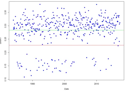
234

235

Figure 2. Graph of SWIR1 band across time. Blue dots represent observed darkness values. The green

236

line is the mean. The red line is -1 standard deviation. TDOM would identify any value below the red

237

line as a dark outlier in the SWIR1 band. This same analysis is then performed in the NIR band to

238

identify dark outliers.

239

This study used the normalized difference vegetation index (NDVI) (equation 6) [22] and the

240

normalized burn ratio (NBR) (equation 7) as indices of forest greenness to detect forest changes [23].

241

= , (6)

= , (7)

(8)

Where NIR is the near infrared band of a multispectral image, red is the red band of a multispectral

243

image, and SWIR2 is the second shortwave infrared band of a multispectral image.

244

245

2.6 Change Detection Algorithms

246

Three algorithms were developed and tested in GEE using MODIS and Landsat data. Employing

247

GEE for this study enabled us to efficiently test various change detection approaches using Landsat

248

and MODIS image data archives, without downloading and storing the data locally.

249

ORS mapping needs fell into two categories - ephemeral change related to defoliation events

250

and long-term change related to tree mortality from insects and disease. The three algorithms used

251

in this study were selected to address the needs posed by these forest change types. We will be

252

referring to these algorithms as: Basic z-score (Figure 3), Harmonic z-score (Figure 4), and Linear

253

trend (Figure 5).

254

The basic z-score method builds on ideas from RTFD, serving as a natural starting point for ORS

255

mapping methods. The harmonic z-score method combines ideas from harmonic regression-based

256

methods, such as EWMACD [12] and BFAST Monitor [11], with those from the basic z-score method

257

to leverage data from throughout the growing season. The linear trend method is built on ideas from

258

Vogelmann et al. [24] and the RTFD trend method [3]. It uses linear regression to fit a line across a

259

series of years.

260

Both the basic z-score and harmonic z-score method work by identifying pixels that differ from

261

a baseline period. The primary difference is what data are used to compute the z-score. Both methods

262

start by acquiring imagery for a baseline period (generally 3-5 years) and analysis years. The basic

z-263

score method uses the mean and standard deviation of the baseline period within a targeted date

264

range for a specified band or index, while the harmonic z-score method first fits a harmonic

265

regression model to all available cloud/cloud shadow-free Landsat or MODIS data.

266

The harmonic regression model is intended to mitigate the impact of seasonality on the spectral

267

response, leaving remaining variation to be related to change unrelated to phenology. The harmonic

268

is defined as:

269

= 0 + 1 + 2 cos(2 )+ 3 sin(2 ) (8)

where b is the band or index of the image, are the coefficients being fit by the model, and t is the

270

sum of the date expressed as a year and the proportion of a year.

271

The harmonic regression model is fitted on a pixel-wise basis to the baseline data and then

272

applied to both the baseline and the analysis data. Next, the residual error is computed for both the

273

baseline and analysis data. The mean and standard deviation of the baseline residuals are used to

274

compute the z-score of the analysis period residuals. Finally, the analysis period residuals are limited

275

to the targeted date period. The date range and specific years used to define the baseline can be

276

tailored to optimize the discernment of specific disturbances within the analysis years.

277

Since an analysis period may have more than a single observation, a method for summarizing

278

these values is specified for both the basic and harmonic score methods to constrain the final

z-279

score value. For this study, the mean of values was used. Change is then identified by thresholding

280

the summary z-score value. For this project, summarized z-score values less than -0.8 were identified

281

as change. This threshold was chosen based on analyst expertise obtained from iterative qualitative

282

comparison of z-score results with post-disturbance image data.

283

(9)

285

Figure 3. Illustration of the basic z-score approach. First observations are limited to a specified date

286

period (July 1- August 31 in this example). The mean and standard deviation of the baseline

287

observations (2011-2015 in this example) are then computed. These statistics are then applied to the

288

analysis year (2016 in this example) to find departures from the baseline.

289

290

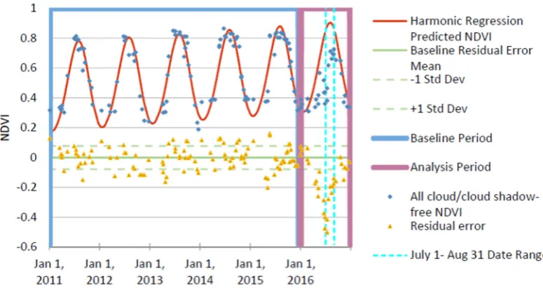
Figure 4. Illustration of the harmonic z-score change detection approach. In order to capture the

291

seasonality of a pixel, this approach uses data from the entire year. A harmonic regression model is

292

first fit to the baseline data (2011-2015 in this example). That same harmonic model is then applied to

293

both the baseline and analysis (2016 in this example) data. The mean and standard deviation of the

294

residual error from the baseline observations are then computed. These statistics are then applied to

295

the residual error of the analysis data to find departures from expected seasonality. Finally, the

296

residual z-score for the analysis data is constrained to the specified date range.

297

The linear trend method first gathers data for a specified number of years prior to the analysis

298

year, referred to as an epoch. For an epoch, an ordinary least square linear regression model is fit on

299

(10)

= + , ₍₉₎

301

where b is the band or index of image, a0 is the intercept, a1is the slope, t is the date, and y is the

302

predicted value.

303

Change is identified where the slope (a1) is less than -0.03- a threshold which was chosen based

304

on analyst expertise similar to the identification of the threshold used for the z-score methods.

305

306

Figure 5. Illustration of the trend change detection algorithm. First observations are limited to a

307

specified date period (July 1- August 31 in this example). Then for a given epoch (2012-2016 in this

308

example) an ordinary least squares linear regression model is fit to the annual median pixel value.

309

The slope of this line is then thresholded to find change areas.

310

We tested all three methods in both study areas. Analysts chose targeted date ranges based on

311

expert knowledge of when each event was most visible.

312

2.7 Accuracy Assessment Methods

313

We performed an independent accuracy assessment to understand how well ORS products

314

performed relative to existing FHP disturbance mapping programs. We followed best practices for

315

sample design, response design, and analysis as outlined in Olofsson et al. [25]. We drew a simple

316

random sample across all 30m x 30m pixels that were within each study area’s tree mask. Since all

317

change detection for this study was performed retrospectively, timely field reference data could not

318

be collected. Instead, we collected independent reference data using TimeSync [13]. TimeSync is a

319

tool that enables a consistent manual inspection of the Landsat time series along with high resolution

320

imagery found within Google Earth. Single Landsat pixel-size (30m x 30m) plots were analyzed

321

throughout the baseline and analysis periods. The response design was created for the US Forest

322

Service Landscape Change Monitoring System (LCMS) [26] and USGS Landscape Change

323

Monitoring Assessment and Projection (LCMAP) [27] projects to provide consistent depictions of

324

land cover, land use, and change process. Rigorous analyst training and calibration was used to

325

overcome the subjective nature of analyzing data in this manner. We analyzed a total of 230 plots

326

across the Rio Grande National Forest and 416 plots across the Southern New England study area.

327

We then cross-walked all responses for each year to change and no change. For consistency, all ORS,

328

IDS, and RTFD outputs had the same 30 meter spatial resolution tree mask applied to them that was

329

(11)

from 250 meter to 30 meter spatial resolution using nearest neighbor resampling. The reference data

331

was then compared to each of the ORS outputs along with the IDS and RTFD products for each

332

analysis year to provide overall accuracy, kappa, and class-wise omission and commission error rates.

333

While this method provides a depiction of the accuracy of the assessed change detection methods

334

within the tree mask, it completely omits any areas outside of this mask from all analyses.

335

336

3. Results

337

The reference dataset produced using TimeSync for each analysis year was compared to each of

338

the 12 ORS outputs, as well as the RTFD and IDS outputs. The 12 ORS outputs reflect the combination

339

of basic z-score, harmonic z-score, and trend analysis methods, calculated using either NDVI or NBR

340

greenness indices, and derived from either Landsat or MODIS data.

341

3.1 Southern New England

342

We collected the following data for the Southern New England analysis:

343

• IDS data were from separate aerial and ground surveys performed in Massachusetts,

344

Connecticut, and Rhode Island from June 7 - August 25, 2016, and June 26 - August 26,

345

2017.

346

• RTFD data were from June 10 - July 27, 2016, and June 26 - August 12, 2017.

347

• ORS analyses were conducted between May 25 and July 9 for both 2016 and 2017.

348

Baseline years spanned from 2011-2015 for harmonic z-score and regular z-score

349

methods while a three year epoch length was used for the linear trend method.

350

The overall accuracy of all outputs ranged from 77.88% to 93.51% (kappa 0.09-0.59) in 2016 and

351

77.64% to 87.02% (kappa 0.12-0.57) in 2017 (Tables 3 and 4). The highest overall accuracy and kappa

352

and lowest commission and omission error rates are highlighted in each table. While the ORS trend

353

algorithm had the highest overall accuracy and kappa for both 2016 and 2017, omission and

354

commission error rates were quite varied and inconsistent across different combinations of algorithm,

355

platform, and index. Most ORS outputs performed as well or better than IDS and RTFD outputs for

356

both years.

357

The patterns of spatial agreement are evident in Figure 6, where a heatmap of the number of

358

ORS outputs that found a pixel as change are displayed with the corresponding IDS and RTFD

(z-359

score) maps. Overall spatial patterns are similar between each product. There is a notable similarity

360

between the RTFD maps and MODIS-based ORS maps. This reflects the similarities between the

361

(12)

Table 3. Southern New England overall accuracy, kappa, and omission/commission error rates for each ORS method tested as well as existing FHP program outputs (IDS

363

and RTFD) for 2016. The highest overall accuracy and kappa and lowest commission and omission error rates are highlighted.

364

ORS Method Platform Index

Overall

Accuracy Kappa

Tree No Change Commission Error Rate

Tree No Change Omission Error Rate

Tree Change Commission Error Rate

Tree Change Omission Error Rate

Harmonic Z-score Landsat NBR 92.79% 0.30 7.33% 0.00% 0.00% 81.08%

Harmonic Z-score Landsat NDVI 92.79% 0.43 6.05% 1.58% 31.58% 64.86%

Harmonic Z-score MODIS NBR 91.59% 0.09 8.45% 0.00% 0.00% 94.59%

Harmonic Z-score MODIS NDVI 91.35% 0.09 8.47% 0.26% 33.33% 94.59%

Basic Z-score Landsat NBR 77.88% 0.36 0.00% 24.27% 71.32% 0.00%

Basic Z-score Landsat NDVI 90.38% 0.52 2.79% 7.92% 52.63% 27.03%

Basic Z-score MODIS NBR 92.07% 0.53 3.99% 4.75% 45.00% 40.54%

Basic Z-score MODIS NDVI 91.35% 0.27 7.23% 1.85% 46.67% 78.38%

Linear Trend Landsat NBR 92.07% 0.59 2.21% 6.60% 46.30% 21.62%

Linear Trend Landsat NDVI 93.51% 0.58 3.93% 3.17% 35.29% 40.54%

Linear Trend MODIS NBR 91.35% 0.55 2.75% 6.86% 49.06% 27.03%

Linear Trend MODIS NDVI 91.83% 0.43 5.66% 3.17% 44.44% 59.46%

RTFD MODIS NDVI 84.86% 0.30 5.11% 11.87% 70.31% 48.65%

IDS -- -- 89.18% 0.32 6.05% 5.80% 61.11% 62.16%

365

366

doi:10.20944/preprints201805.0360.v1

Peer-reviewed version available at

Remote Sens.

2018

,

10

, 1184;

(13)

Table 4. Southern New England overall accuracy, kappa, and omission/commission error rates for each ORS method tested as well as existing FHP program outputs

367

(IDS and RTFD) for 2017. The highest overall accuracy and kappa and lowest commission and omission error rates are highlighted.

368

369

Overall

Accuracy Kappa

Harmonic Z-score Landsat NBR 84.13% 0.27 15.23% 1.76% 27.27% 78.95%

Harmonic Z-score MODIS NBR 83.41% 0.14 16.87% 0.00% 0.00% 90.79%

Linear Trend Landsat NBR 87.98% 0.61 6.33% 8.53% 34.52% 27.63%

Linear Trend Landsat NDVI 81.97% 0.46 8.20% 14.41% 49.49% 34.21%

Linear Trend MODIS NBR 87.02% 0.57 7.94% 7.94% 35.53% 35.53%

RTFD MODIS NDVI 84.38% 0.43 11.27% 7.35% 40.98% 52.63%

IDS -- -- 79.81% 0.41 8.97% 16.47% 53.85% 36.84%

370

doi:10.20944/preprints201805.0360.v1

Remote Sens.

2018

,

10

, 1184;

(14)

371

Figure 6. Map panels showing the extent of gypsy moth defoliation within the Southern New England

372

study area in 2016 and 2017 as depicted by the RTFD analytical output, the IDS database, and ORS

373

MODIS and Landsat analyses. ORS outputs are presented as heatmaps of the number of outputs that

374

(15)

3.4 Rio Grande National Forest

376

The southwestern United States, including the Rio Grande National Forest study area, has been

377

impacted for the last 20 years by prolonged drought conditions, contributing to slow-onset insect

378

infestations including mountain pine beetle and spruce bark beetle [24, 28]. This study focused on the

379

change that occurred in 2013 and 2014.

380

We collected the following data for the analysis:

381

• IDS data were from a wall-to-wall aerial survey of forested areas in Colorado, which

382

were conducted from July 30 to September 18, 2013 and June 24 to September 3, 2014.

383

• RTFD data were from July 28 to August 28 for both analysis years.

384

• ORS analyses were conducted from July 9 to October 15 for 2013 and 2014. Baseline years

385

spanned from 2007-2011 for harmonic z-score and regular z-score methods while a five

386

year epoch length was used for the linear trend method.

387

The overall accuracy of products obtained for the Rio Grande study area were a bit lower than

388

the Southern New England study area- ranging from 71.30% to 79.57% (kappa 0.12-0.42) in 2013 and

389

59.57% to 76.09% (kappa -0.09-0.45) in 2014 (Tables 5 and 6). Much like the results from Southern

390

New England, results varied across the different combinations of algorithm, platform, and index. In

391

general, the linear trend ORS method performed the best for both the 2013 and 2014 outputs. This is

392

not surprising due to the gradual nature of tree decline and mortality caused by the bark beetle

393

disturbance that has been occurring in this study area.

394

The heatmap in Figure 7 shows different patterns of spatial agreement and disagreement than

395

we observed in the Southern New England study area. The first notable difference is that both RTFD

396

and ORS methods continue to capture areas that changed in both 2013 and 2014, while IDS maps only

397

show new areas of change in 2014. This difference is inherent in the underlying methods, as IDS will

398

often not remap previously existing long-term change. The second notable difference is that the area

399

of new tree change in 2014 in the northeast portion of the study area was largely missed by RTFD,

400

(16)

Table 5. Rio Grande study area overall accuracy, kappa, and omission/commission error rates for each ORS method tested as well as existing FHP program outputs- IDS

402

and RTFD for 2013. The highest overall accuracy and kappa and lowest commission and omission error rates are highlighted.

403

404

Overall

Accuracy Kappa

Harmonic Z-score MODIS NBR 77.83% 0.42 14.71% 15.20% 43.33% 42.37%

Linear Trend Landsat NBR 78.26% 0.42 15.03% 14.04% 42.11% 44.07%

Linear Trend Landsat NDVI 79.57% 0.33 20.19% 2.92% 22.73% 71.19%

RTFD MODIS NDMI 71.30% 0.12 23.35% 11.70% 60.61% 77.97%

IDS -- -- 75.65% 0.29 19.58% 11.11% 46.34% 62.71%

405

406

doi:10.20944/preprints201805.0360.v1

Remote Sens.

2018

,

10

, 1184;

(17)

Table 6. Rio Grande study area overall accuracy, kappa, and omission/commission error rates for each ORS method tested as well as existing FHP program outputs- IDS

407

and RTFD for 2014. The highest overall accuracy and kappa and lowest commission and omission error rates are highlighted.

408

409

Overall

Accuracy Kappa

Harmonic Z-score MODIS NBR 73.48% 0.36 19.02% 18.52% 44.78% 45.59%

Harmonic Z-score MODIS NDVI 59.57% -0.09 31.55% 20.99% 79.07% 86.76%

Basic Z-score MODIS NBR 76.09% 0.40 19.08% 13.58% 38.60% 48.53%

Linear Trend Landsat NBR 76.09% 0.45 15.03% 19.75% 41.56% 33.82%

Linear Trend Landsat NDVI 74.78% 0.21 25.93% 1.23% 14.29% 82.35%

Linear Trend MODIS NDVI 76.09% 0.30 23.65% 4.32% 25.93% 70.59%

RTFD MODIS NDMI 71.74% 0.14 27.01% 4.94% 42.11% 83.82%

IDS -- -- 67.83% 0.15 26.09% 16.05% 56.52% 70.59%

410

doi:10.20944/preprints201805.0360.v1

Remote Sens.

2018

,

10

, 1184;

(18)

411

Figure 7. Map panels showing the extent of mountain pine beetle and spruce budworm damage

412

within the Rio Grande National Forest study area in Colorado in 2013 and 2014 as depicted by the

413

RTFD analytical output, the IDS database, and ORS MODIS and Landsat analyses. ORS outputs are

414

presented as heatmaps of the number of outputs that found the area as change (1-6).

415

416

(19)

4. Discussion

418

This study improves our understanding of how well ORS algorithms perform compared to

419

existing FHP mapping programs. Some differences between spatial data from the IDS, RTFD, and

420

ORS maps are inherent to the missions of these programs, while other differences are related to

421

disparate approaches used to create the data. Due to the ephemeral nature of the Eastern defoliation

422

events and ongoing gradual mortality occurring in the Western beetle infestation that were the target

423

of this investigation, field-based reference data did not exist. Future studies that collect ground-based

424

field observations would be a valuable independent comparator for ORS maps.

425

Various accuracy measures demonstrated that ORS outputs generally performed comparably or

426

better than IDS or RTFD products. IDS and RTFD data generally depict change at a coarse spatial

427

scale, limiting its potential accuracy when compared to reference data assessed at the Landsat spatial

428

scale.

429

Additional differences between Landsat and MODIS relate to their temporal resolution. The

430

limited availability of cloud/cloud shadow-free Landsat images hinders its utility to detect ephemeral

431

forest disturbances that must be captured within narrow time windows. The frequent observations

432

from MODIS permit a much greater opportunity to detect such disturbances.

433

ORS methods differ from existing RTFD methods in several key areas. Firstly, RTFD products

434

are created in a near-real time environment that GEE cannot currently provide. The composites that

435

are used are therefore slightly different than those used in ORS. Secondly, all baseline statistics are

436

computed on a pixel-wise basis for ORS methods, while they are computed on a zone-wise basis for

437

RTFD methods - where the zones are defined by the combination of USGS mapping zone, forest type,

438

and MODIS look angle strata [3]. This introduces the potential for significant differences in the

439

outputs. The most pronounced difference, however, is that all model input parameters for RTFD are

440

fixed, while ORS parameters can be tailored to a specific forest disturbance event by an expert user.

441

While this introduces the potential for inconsistencies between iterations of ORS, the tool was

442

designed to conduct site-specific targeted change detection in areas already known to have

443

undergone change. Future work to quantitatively optimize the parameters used in ORS algorithms

444

will be conducted.

445

Differences between ORS data and RTFD forest change data are also a result of the disparate

446

objectives of these two programs of work. Specifically, the spatial data created for the RTFD program

447

are not intended to be used as a spatially accurate representation of forest change, but rather as a

448

time-sensitive alarm that forest change is occurring in general areas. These data are very conservative

449

in their spatial representation of forest change, because errors of commission are considered more

450

counterproductive than errors of omission when providing time sensitive spatial information for

451

forest survey mission planning. In contrast, ORS data are intended to act as a spatially accurate

452

representation of forest disturbances. The fundamental goal of the ORS program is to augment the

453

IDS database where data from aerial or ground surveys are not available. As such, intrinsic

454

disagreements between these two spatial data sources are to be expected.

455

Distinctions in observational platform and methodological approach result in differences

456

between spatial data created using ORS algorithms and data from the IDS program. Firstly, whereas

457

the ORS and RTFD change data are derived from space-borne satellite imagery from Landsat and

458

MODIS platforms, the IDS data are derived from observations made by state and local forestry

459

personnel from ground surveys or an aerial vehicle (e.g., fixed-wing aircraft or helicopter). Secondly,

460

there is a range of methods used to compile IDS data on a state-by-state basis. The inconsistent

461

methods employed to produce IDS data on a local level are evident in the Southern New England

462

study area, where large polygons are favored in Massachusetts, smaller polygons are more common

463

in Connecticut, and grid cells are the primary spatial unit in Rhode Island (Figure 8). In contrast, the

464

results obtained from forest change detection algorithms using satellite imagery do not vary from

465

place to place, but rather maintain an objective quality over space and time. This is a primary reason

466

why varying levels of agreement were seen between IDS data with the ORS and RTFD spatial results

467

(20)

469

Figure 8. Map of the 2017 IDS spatial data used for the Southern New England study area depicting

470

three different methods of IDS delineation- large polygons in MA, small polygons in CT, and grid

471

cells in RI.

472

This study did not make use of Sentinel-2 Multispectral Instrument data, as its availability

473

remains sparse over North America. These data are also freely available, regularly collected, and have

474

similar spatial resolution and spectral response functions to those of Landsat [29]. The spatial and

475

spectral similarity of Sentinel and Landsat suggests that these image data could be combined for

476

hybrid analyses. Future work that incorporates these data to create ORS products will likely improve

477

the quality of non-MODIS-based outputs by providing more temporally dense data to detect and

478

track ephemeral forest disturbances.

479

5. Conclusions

480

This study tested three algorithms developed to map forest change for the USDA Forest Service’s

481

FHP. Utilizing GEE as a platform to create these spatial data products was efficient and effective. The

482

ORS spatial data had similar or higher accuracy than existing FHP mapping program outputs. A

483

unique strength of ORS spatial data lies in the adaptive nature of the algorithms employed. In

484

contrast to the standardized method employed to create data for the RTFD program, the ability to

485

adjust model parameters based on the characteristics of specific disturbance events permits the

486

tuning of ORS spatial products. Additionally, the flexibility to use either Landsat scale or MODIS

487

satellite image data in ORS algorithms permits the collection of timely synoptic observations

488

regardless of the ephemeral nature of intra-seasonal forest disturbances.

489

This study demonstrates the utility of ORS methods for spatially characterizing ephemeral as

490

well as long term forest disturbances. These data have been used to augment the 2017 annual IDS

491

database in the Southern New England study area for disturbances that occurred after the annual

492

ADS had concluded [30]. In future years, data from ORS models will also be used to respond to local

493

disturbance reports from counties, states, and forest units.

494

Acknowledgments: This research was performed under contract to the US Forest Service, Geospatial

495

Technology and Applications Center (GTAC) and in support of applications being developed for the Forest

496

Health Assessment and Applied Sciences Team (FHAAST). We are grateful for their support and this important

497

(21)

Earth Engine team - specifically Noel Gorelick and Matthew Hancher - in the design, execution, and analysis

499

using Earth Engine. Lastly, we wish to acknowledge the many useful contributions of other RedCastle Resources

500

and Forest Service technical personnel. Three anonymous reviewers also offered helpful critique and valuable

501

recommendations for this paper.

502

References

503

1. United States Department of Agriculture. Detection Surveys Overview. Available online:

504

https://www.fs.fed.us/foresthealth/technology/detection_surveys.shtml (accessed on September 19, 2017).

505

2. United States Department of Agriculture. FY10 Mishap Review. Available online:

506

https://www.fs.fed.us/fire/av_safety/assurance/mishaps/,

507

https://www.fs.fed.us/fire/av_safety/assurance/mishaps/FY10_Mishap_Review.pdf (accessed on

508

September 21, 2017).

509

3. Chastain, R.A.; Fisk, H.; Ellenwood, J.R.; Sapio, F.J.; Ruefenacht, B.; Finco, M.V.; Thomas, V. Near-real time

510

delivery of MODIS-based information on forest disturbances. In Time Sensitive Remote Sensing, Lippitt, C.D.,

511

Stow, D.A., Coulter L.L. Eds.; Springer: New York, USA, 2015, pp. 147-164, ISBN 978-1-4939-2601-5.

512

4. Coppin, P.R.; Bauer, M.E. Change detection in forest ecosystems with remote sensing digital imagery. Rem

513

Sens Reviews 1996, 13, 207-234.

514

5. Lu, D.; Mausel, P.; Brondizio, E.; Moran, E. Change detection techniques. Int Jour Rem Sens 2004, 25,

2365-515

2407, doi:10.1080/0143116031000139863.

516

6. Huang, C.; Goward, S.; Masek, J.; Thomas, N.; Zhu, Z.; Vogelmann, J. An automated approach for

517

reconstructing recent forest disturbance history using dense Landsat time series stacks. Rem Sens Env 2010,

518

114, 183-198, doi:10.1016/j.rse.2009.08.017.

519

7. Kennedy, R.; Yang, Z.; Cohen, W. Detecting trends in forest disturbance and recovery using Landsat time

520

series: 1. LandTrendr - Temporal segmentation algorithms. Rem Sens Env 2010, 114, 2897-2910,

521

doi:10.1016/j.rse.2010.07.008.

522

8. Verbesselt, J.; Hyndman, R.; Newnham, G.; Culvenor, D. Detecting trend and seasonal changes in satellite

523

image time series. Rem Sens Env 2010, 114, 106-115, doi:10.1016/j.rse.2009.08.014.

524

9. Stueve, K.M.; Housman, I.W.; Zimmerman, P.L.; Nelson,M.D.; Webb, J.B.; Perry, C.H.; et al. Snow-covered

525

Landsat time series stacks improve automated disturbance mapping accuracy in forested landscapes. Rem

526

Sens Env 2011, 115, 3203–3219, doi:10.1016/j.rse.2011.07.005.

527

10. Zhu, Z.; Woodcock, C. Continuous change detection and classification of land cover using all available

528

Landsat data. Rem Sens Env 2014, 144, 152-171, doi:10.1016/j.rse.2014.01.011.United States Department of

529

Agriculture. Detection Surveys Overview. Available online:

530

https://www.fs.fed.us/foresthealth/technology/detection_surveys.shtml (accessed on September 19, 2017).

531

11. Verbesselt, J.; Zeileis, A.; Herold, M. Near real-time disturbance detection using satellite image time series.

532

Rem Sens Env 2012, 123, 98-108, doi:10.1016/j.rse.2012.02.022.

533

12. Brooks, E.B.;Wynne, R.H.; Thomas, V.A.; Blinn, C.E.; Coulston, J.W. On-the-Fly massively multitemporal

534

change detection using statistical quality control charts and Landsat data. IEEE Trans Geosci Rem Sens 2013,

535

52, 3316-3332, doi:10.1109/TGRS.2013.2272545.

536

13. Cohen, W.B.; Yang, Z.; Kennedy, R. Detecting trends in forest disturbance and recovery using yearly

537

Landsat time series: 2. TimeSync – tools for calibration and validation. Rem Sens Env 2010, 114, 2911-2924,

538

doi:10.1016/j.rse.2010.07.008.

539

14. Griffiths, P.; Kuemmerle, T.; Kennedy, R.E.; Abrudan, I.V.; Knorn, J.; Hostert, P. Using annual time-series

540

of Landsat images to assess the effects of forest restitution in post-socialist Romania. Rem Sens Env2012,

541

118, 199-214, doi:10.1016/j.rse.2011.11.006.

542

15. Cohen, W.B.; Healy, S.P.; Yang, Z.; Stehman, S.V.; Brewer, C.K.; et al. How similar are forest disturbance

543

maps derived from different Landsat time series algorithms? Forests 2017, 8, 98-117, doi: 10.3390/f8040098.

544

16. United States Forest Service. Available online:

545

https://www.fs.usda.gov/detailfull/riogrande/home/?cid=stelprdb5409285&width=full (accessed on May

546

15, 2018).

547

17. Ruefenacht, B.; Benton, R.; Johnson, V.; Biswas, T.; Baker, C.; Finco, M.; Megown, K.; Coulston, J.;

548

Winterberger, K.; Riley, M. Forest service contributions to the national land cover database (NLCD): Tree

549

Canopy Cover Production. In Pushing boundaries: new directions in inventory techniques and

550

(22)

2015; Stanton, S.M., Christensen, G,A., Eds. U.S. Department of Agriculture, Forest Service, Pacific

552

Northwest Research Station, 2015; Gen. Tech. Rep. PNW-GTR-931, pp. 241-243.

553

554

18. Johnson, E.W.; Wittwer, D. Aerial Detection Surveys in the United States. In: Aguirre-Bravo, C.; Pellicane,

555

Patrick J.; Burns, Denver P.; and Draggan, Sidney, Eds. 2006. Monitoring Science and Technology

556

Symposium: Unifying Knowledge for Sustainability in the Western Hemisphere Proceedings

RMRS-P-557

42CD. Fort Collins, CO: U.S. Department of Agriculture, Forest Service, Rocky Mountain Research Station,

558

2006, pp. 809-811.

559

560

19. Chander, G.; Markham, B.L.; Helder, D.L. Summary of current radiometric calibration coefficients for

561

Landsat MSS, TM, ETM+, and EO-1 ALI sensors. Rem Sens Env 2009, 113, 893-903,

562

doi:10.1016/j.rse.2009.01.007.

563

20. Gorelick, N.; Hancher, M.; Dixon, M.; Ilyushchenko, S.; Thau, D.; Moore, R. Google Earth Engine:

Planetary-564

scale geospatial analysis for everyone. Rem Sens Envin press, doi:10.1016/j.rse.2017.06.031.

565

21. Housman, I.; Hancher, M.; Stam, C. A quantitative evaluation of cloud and cloud shadow masking

566

algorithms available in Google Earth Engine. Manuscript in preparation.

567

22. Rouse, J.W.; Haas, R.H., Jr.; Schell, J.A.; Deering, D.W. Monitoring vegetation systems in the Great Plains

568

with ERTS. Third ERTS-1 Symposium, Washington, DC, USA, 1974, pp. 309–317.

569

23. Key, C.H.; Benson, N.C. Landscape Assessment: Ground measure of severity, the composite burn index;

570

and remote sensing of severity, the Normalized Burn Ratio, 2006. USDA Forest Service, Rocky Mountain

571

Research Station, Ogden, UT. RMRS-GTR-164-CD: LA 1-51. Available at:

572

http://pubs.er.usgs.gov/publication/2002085

573

574

24. Vogelmann, J.; Xian, G.; Homer, C.; Tolk, B. Monitoring gradual ecosystem change using Landsat time

575

series analyses: Case studies in selected forest and rangeland ecosystems. Rem Sens Env 2012, 12, 92-105,

576

doi:10.1016/j.rse.2011.06.027.

577

25. Olofsson, P.; Foody, G.M.; Herold, M.; Stehman, S.; Woodcock, C.E.; Wulder, M.A. Good practices for

578

estimating area and assessing accuracy of land change. Rem Sens Env 2014, 148, 42-57,

579

doi:10.1016/j.rse.2014.0.015.

580

26. Healy, S.P.; Cohen, W.B.; Yang, Z.; Brewer, K.; et al. Mapping forest change using stacked generalization:

581

An ensemble approach. Rem Sens Env 2018, 204, 717-728, doi:10.1016/j.rse.2017.09.029.

582

27. Pengra, B.; Gallant, A.L.; Zhu, Z.; Dahal, D. Evaluation of the initial thematic output from a continuous

583

change-detection algorithm for use in automated operational land-change mapping by the U.S. Geological

584

Survey. Rem Sens 2016, 8, 811-843, doi:10.3390/rs8100811.

585

28. Williams, A.P.; Allen, C.D.; Millar, C.I.; Swetman, T.W.; Michaelson, J.; Still, C.J.; Leavitt, S.W. Forest

586

responses to increasing aridity and warmth in the southwestern United States. PNAS 2010, 107,

21289-587

21294, doi:10.1073/pnas.0914211107.

588

29. United States Geological Survey. Available online: https://landsat.usgs.gov/using-usgs-spectral-viewer

589

(accessed on August 5, 2017).

590

30. Thomas, V. (Forest Health Assessment and Applications Sciences Team, Fort Collins, CO, USA). Personal

591

Creative Commons CC BY

, 1184; doi:10.3390/rs10081184