From Stochastic Geometry to Structural Access Point
Deployment for Wireless Networks: A Lloyd
Algorithm Approach
Ali Rıza Ekti
Balıkesir University, Department of Electrical and Electronics Engineering, Balıkesir, Türkiye; [email protected]
Abstract:In a wireless network, locations of base stations (BSs)/access points (APs)/sensor nodes can
be modeled based on stochastic processes, e.g., a Poisson point process (PPP) or a deterministic pattern planned ahead by providers. While deterministic deployment does not provide tractable interference analysis in general, PPP yields tractable analysis for interference. However, PPP allows APs to be deployed very close to each other and gives pessimistic results compared to the field measurements. In this study, in order to address this issue, Lloyd’s algorithm, which functions as a bridge between random and structural APs deployments, is investigated for analyzing coverage probability in a network. The link distance distribution is modeled as a mixture of Weibull distributions and its parameters are obtained by using the expectation-maximization (EM) algorithm for each iteration of Lloyd’s algorithm. The link distance distribution is further utilized for calculating the coverage probability approximately by exploiting the tractability of PPP.
Keywords:Expectation-maximization algorithm; Lloyd’s algorithm; stochastic geometry; Poisson
point process; Voronoi diagram
0. Introduction
Rapidly accumulating device diversity, user demands, and need for better coverage make network planning more complicated and introduce randomness in the deployment of BSs/APs. In the scenarios where the locations of BSs/APs do not follow a deterministic structure, modeling the performance of the network precisely becomes a challenging task. One of the proposed approaches is to model BS/AP deployment as an independent PPP, a methodology which provides analytical tractability for interference and coverage probability analyses [1,2]. However, the independent PPP assumption ignores the correlation among the BSs/APs. Field measurements show that the coverage probability lies in practice between the traditional hexagonal model and the independent PPP approach. This is mainly due to the fact that network operators have still control on BS/AP deployment in a deterministic way [3,4], which creates intentional repulsion between BSs/APs. Therefore, more realistic ways should be incorporated while still maintaining the tractability of PPP for interference analysis. The authors in [5,6] apply aα-Ginibre point process (GPP) and aβ-GPP to model the correlation between BSs/APs. The GPP is a deterministic point process and takes into account the repulsion between BSs/APs.
In this study, we investigate scenarios where BSs/APs are deployed neither totally random nor totally deterministic. We propose a semi-analytical strategy by adopting the Lloyd’s algorithm to account for the scenarios that lie between the pessimistic PPP-based deployment and the optimistic structural BS/AP deployment. We derive the link distance distribution for each iteration of Lloyd’s algorithm by using the EM algorithm. It is shown that the link distance can be approximated well by a mixture of Weibull distributions. By integrating the link distance distribution into the PPP analysis, we provide a coverage probability analysis.
The rest of the paper is organized as follows. The Lloyd’s algorithm is described in Section1. The analysis of link distance distribution is given in Section2. Section3presents the coverage probability
study. The numerical results are presented in Section4. The concluding remarks are provided in Section5.
1. Lloyd’s Algorithm Approach
A two-dimensional (2D) Voronoi diagram is a tessellation in which each polygon depicts the set of points nearest to a central generator point. Voronoi diagrams present diverse applications in many fields such as wireless communications, astronomy, archeology, physics, mathematics, and coding [7,8]. Lloyd’s algorithm incrementally moves the generator of each polygon to the centroid of that polygon and maximizes the distance between adjacent generators [9]. The maximization procedure creates repulsion between adjacent generators until the generators establish a fixed state such as centroidal Voronoi tessellation (CVT). The resultant Voronoi diagram gives a structural geometry asymptotically, depending on how many iteration steps are used [10]. The centroid of each Voronoi cell is given for each iteration by
Ci =
R
Arλ(r)dA
R
Aλ(r)dA
. (1)
Ciis the centroid of the Voronoi cell,ris the position andλ(r)denotes the intensity ofrandAstands
for the area. Lloyd’s Algorithm
1. Choose N points andCi ⊂R
2. ∀ni ∈ NfindCithe closest center and repeat until the Euclidian distance betweenCiandNi
equals to zero.
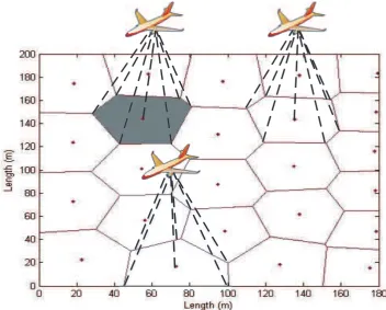
In this study, we initialize the tessellation of BSs/APs based on a PPP. While the initial geometry captures the randomness of BS/AP deployment, the asymptotic Voronoi diagram with Lloyd’s algorithm yields a structural BS/AP deployment. Each iteration of the Lloyd’s algorithm represents an intermediate deployment scenario between the random and structural BS/AP deployments, which motivates us to adopt Lloyd’s algorithm for modeling BS/AP deployment. A demonstration of iteration steps {0, 9, 490} is illustrated in Fig.1. Furthermore, BSs/APs and/or sensors can be placed on the drones, i.e., autonomous planes, and drones can give coverage to areas such as disaster/public safety regions, rural areas and downtown areas as seen in Fig.2. We can also utilize it for the self organized networks (SON) networks to decide the best coverage options for a given area. Hence, to exploit Lloyd’s algorithm for modeling BS/AP and/or sensor deployment, the analytical expression of link distance distribution at each iteration of Lloyd’s algorithm is required. To the best of our knowledge, the link distance distribution is not available in the literature, and an approximate distribution is derived in the next section by exploiting the EM algorithm.
2. Link Distance Distribution Analysis
0 50 100 150 200 0
20 40 60 80 100 120 140 160 180 200
Length (m)
Length (m)
(a) Iteration 0.
0 50 100 150 200
0 20 40 60 80 100 120 140 160 180 200
Length (m)
Length (m)
(b) Iteration 9.
0 50 100 150 200
0 20 40 60 80 100 120 140 160 180 200
Length (m)
Length (m)
(c) Iteration 490.
Figure 1.Illustration of transition from random BS/AP deployment to structural BS/AP deployment
with the Lloyd’s algorithm.
Figure 2.Drone integrated system illustration.
fr(r) = dFr
(r)
dr =
d
dr(1−P[r>R])
= d
dr(1−P[No BS closer than R])
= d
dr 1− (λA)0
0! e −λA
!
= d
dr
1−e−λA
= d
dr
1−e−λπR2
= e−λπr22
which corresponds to a Rayleigh distribution with variance 1/2λπ. On the other hand, considering the case of hexagonal tessellation, the PDF of link distance is given by [11]
fr(r) =
πr √
3R2, 0≤r≤R.
2√3r R2
h
π
6 −cos−1
R r
i
, R≤r≤ 2R
√
3 3 .
0, r≥ 2R√3
3 .
(3)
The transition from (2) to (3) via Lloyd’s algorithm can be approximated as a mixture of Weibull distributions by employing the EM algorithm. A mixture of Weibull distributions can be expressed as
fr(r) = l
∑
j=1φj ϕj δj r δj
!ϕj−1
e
−δr
j
ϕj
, (4)
whereφj is the weight ofjth component and∑lj=1φj =1,δjandϕjare the scale parameter and the
shape parameter, respectively, andlis the number of Weibull distributions. In order to consider various BS/AP intensities, we defineδjto beψj
√
λ0/λ, whereλ0is a constant andψjis the scale parameter
when λ = λ0. The main reasons for using a mixture of Weibull distributions are: (i) Rayleigh
distribution is a special case of a Weibull distribution if the Weibull parameters are properly selected, (ii) The support of Weibull distribution is[0,∞], and (iii) Weibull distribution can provide negative and positive skewness, a feature required in the transitions from (2) to (3). Next, we discuss the calculations of parametersφj,δjandϕjwith the EM algorithm.
2.1. EM Algorithm for Link Distance Distribution
We have a training set r = {r(1),r(2),· · ·,r(m)} consisting of m independent observations
generated by considering each iteration step of Lloyd’s algorithm. Our goal is to fit the Weibull parameters to the link distance distribution by utilizing the EM algorithm. The EM algorithm consists of two steps, namely, the expectation (E)-step and the maximization (M)-step. The reader is referred to [12] for more detailed explanations about the EM algorithm.
The complete log-likelihood is defined as
L(wj,θ) = m
∑
i=1l
∑
j=1w(ji)log ϕj δj ri δj
!ϕj−1
exp(−r
ϕj
i
δjϕj )φj
, (5)
whereθ={ϕj,δj,φj}andwj(i)=p(z(i)=j|r(i);θ)denotes the posterior probabilities associated with
the hidden label informationz(i). The steps of the EM algorithm are:
• E-step: Choosewjto maximizeL(wj,θ)
wtj=arg max
wj
L(wj,θt).
• M-step: Chooseθto maximizeL(wj,θ)
θt+1=arg max θ
L(wtj,θ).
Maximizing (5) with respect to the parametersϕjandδj, we obtain (6) and (7), respectively
∇ϕL(wj,θ) = m
∑
i=1l
∑
j=1w(ji) 1 ϕj
+ 1− ri
δj
!ϕj! log(ri
δj
) !
, (6)
∇δL(wj,θ) = m
∑
i=1l
∑
j=1w(ji) −ϕj
δj
+ϕj δj
ri
δj
!ϕj!
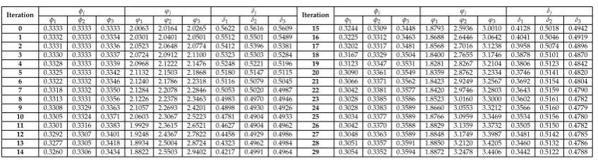
Table 1.Numerical Values ofφj,ϕjandδjas outputs of EM algorithm.
Iteration φj ϕj δj Iteration φj ϕj δj
φ1 φ2 φ3 ϕ1 ϕ2 ϕ3 δ1 δ2 δ3 φ1 φ2 φ3 ϕ1 ϕ2 ϕ3 δ1 δ2 δ3
0 0.3333 0.3333 0.3333 2.0063 2.0164 2.0265 0.5622 0.5616 0.5609 15 0.3244 0.3309 0.3448 1.8793 2.5936 3.0010 0.4128 0.5018 0.4942
1 0.3332 0.3333 0.3334 2.0301 2.0401 2.0501 0.5512 0.5501 0.5489 16 0.3225 0.3312 0.3463 1.8688 2.6446 3.0642 0.4041 0.5046 0.4919
2 0.3331 0.3333 0.3336 2.0523 2.0648 2.0774 0.5412 0.5396 0.5381 17 0.3202 0.3317 0.3481 1.8568 2.7016 3.1238 0.3958 0.5074 0.4896
3 0.3330 0.3333 0.3337 2.0724 2.0912 2.1100 0.5323 0.5303 0.5284 18 0.3167 0.3329 0.3504 1.8400 2.7655 3.1746 0.3878 0.5101 0.4870
4 0.3328 0.3333 0.3339 2.0968 2.1222 2.1476 0.5248 0.5221 0.5196 19 0.3123 0.3347 0.3531 1.8281 2.8267 3.2104 0.3806 0.5123 0.4842
5 0.3325 0.3333 0.3342 2.1132 2.1503 2.1868 0.5180 0.5147 0.5115 20 0.3090 0.3361 0.3549 1.8359 2.8762 3.2334 0.3746 0.5141 0.4820
6 0.3322 0.3332 0.3346 2.1240 2.1786 2.2318 0.5116 0.5079 0.5045 21 0.3066 0.3371 0.3562 1.8423 2.9249 3.2567 0.3692 0.5154 0.4804
7 0.3318 0.3332 0.3350 2.1284 2.2078 2.2846 0.5053 0.5020 0.4987 22 0.3042 0.3381 0.3577 1.8420 2.9746 3.2803 0.3643 0.5159 0.4790
8 0.3313 0.3331 0.3356 2.1226 2.2378 2.3463 0.4983 0.4970 0.4946 23 0.3028 0.3385 0.3586 1.8523 3.0160 3.3000 0.3602 0.5161 0.4782
9 0.3308 0.3329 0.3363 2.1057 2.2693 2.4201 0.4898 0.4930 0.4926 24 0.3028 0.3383 0.3589 1.8660 3.0553 3.3212 0.3566 0.5160 0.4779
10 0.3305 0.3324 0.3371 2.0603 2.3067 2.5223 0.4781 0.4904 0.4933 25 0.3034 0.3377 0.3589 1.8766 3.0959 3.3469 0.3534 0.5156 0.4780
11 0.3301 0.3316 0.3383 1.9929 2.3615 2.6521 0.4627 0.4904 0.4962 26 0.3042 0.3370 0.3588 1.8829 3.1359 3.3732 0.3505 0.5150 0.4782
12 0.3292 0.3307 0.3401 1.9248 2.4367 2.7822 0.4458 0.4929 0.4986 27 0.3048 0.3363 0.3589 1.8848 3.1749 3.3987 0.3481 0.5142 0.4785
13 0.3277 0.3305 0.3418 1.8934 2.5004 2.8724 0.4323 0.4962 0.4984 28 0.3051 0.3357 0.3591 1.8850 3.2120 3.4205 0.3460 0.5132 0.4786
14 0.3260 0.3306 0.3434 1.8822 2.5503 2.9402 0.4217 0.4991 0.4964 29 0.3054 0.3352 0.3594 1.8872 3.2478 3.4406 0.3442 0.5122 0.4788
In order to maximize (5) with respect toφjwhen∑lj=1φj =1, the Lagrangian function is constructed
as
Λ(φj) = m
∑
i=1l
∑
j=1w(ji)logφj+h l
∑
j=1φj−1
!
, (8)
wherehstands for a Lagrange multiplier. After taking the derivative of (8) with respect toφjand
equating it to zero, we obtain:
φj=
1 m
m
∑
i=1w(ji). (9)
An iterative method such as Limited Broyden-Fletcher-Goldfarb-Shanno (L-BGFS) can be applied to obtainϕjandδj[13] due to the fact thatϕjandδjin (6) and (7) do not have explicit forms.
3. Coverage Probability
Probability of coverage is the ratio of the network area where signal-to-interference-noise ratio (SINR) is greater than a certain thresholdTto the total area. It can be defined as
pc(T,λ,α)=4P[SINR>T] =P
hr−α σ2+Ir
>T
, (10)
whereα ≥ 2 is the path loss exponent,h denotes the channel gain between tagged BS/AP and its user, andσ2is the noise power. VariableIrstands for the total interference power received from the
neighboring BSs/APs and is given by
Ir =
∑
n∈Φ/bognR−nα, (11)
wherebo is the tagged BS/AP, gn and Rn are the channel gain and the distance between the nth
interfering BS/AP and the tagged user, respectively. Assuming that the channel gains are characterized with i.i.d. exponential distributions whereE[h] =E[gn] =µ, (10) is expressed as
pc(T,λ,α) = Er[P[SINR>T|r]] =
Z
r>0P
[SINR>T|r] fr(r)dr
= Z
r>0P
hr−α σ2+Ir
>T|r
fr(r)dr
= Z
r>0P
h
h>Tσ2+Ir
rαif
r(r)dr
= Z
r>0e
−µTrασ2L
whereLIr(·)is the Laplace transform ofIrand is given by LIr(µTr
α) =
EIr
h
e−µTrαIri =EΦ,gn
h
e−µTrα∑n∈Φ\b0gnR−nαi. (13)
Due to the independence of fading coefficients, (13) can be re-written as
LIr(µTr α) =
EΦ
∏
n∈Φ\b0
Eg[exp −µTrαgR−nα]
. (14)
By considering the properties of probability generating functional (PGFL) [1,14, ch.4, p.126], (14) can be expressed as
LIr(s) =exp
−2πλ Z ∞
r 1
−Eg[exp(−sgk−α)]kdk
,
=exp
−2πλ Z ∞
0
Z ∞
r
1−e−sk−αgkdk
f(g)d(g)
. (15)
Plugging (4) and (15) into (12), and using the substitutionrϕ=u, the coverage probability is expressed
as
pc(T,λ,α) (16)
=
l
∑
j=1 φj ϕj Z ∞ 0 e λπu ϕj 2
j (1−β(T,α))−µTu
ϕj α j − uj δ ϕj j du j , where
β(T,α) = 2(µT) 2
α
α E
g2αΓ
−2
α,gµT
−Γ
−2
α, 0
andΓ(c,b)stands for the incomplete Gamma function.
4. Numerical Results
In this section, we evaluate Lloyd’s algorithm approximation for coverage probability with computer simulations. BSs/APs are arranged according to a homogeneous PPP in a 300×300 square meter area whereλ=1 unless other stated. We consider a 75×75 square meter in the middle of the total coverage area to eliminate the boundary effect [1]. We consider a Rayleigh fading channel and setαto be 4. The parametersϕj,δj, andφjare provided in TABLE1by using the EM algorithm when
l=3,m=104, andλ0=λ=1. It is worth emphasizing that mixture of three Weibull distributions is sufficient to characterize the link distance distribution. The values in the TABLE1are employed in the calculation of coverage probability.
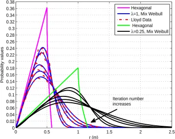
In Fig.3, the link distance distribution is investigated whenλ=1 andλ =0.25. The mixture of Weibull distributions obtained via the EM algorithm agrees with the results of Lloyd’s algorithm. Lloyd’s algorithm performs like a bridge between (2) and (3). The radius of each Voronoi cell becomes evenly distributed as a result of increase in the iteration values, therefore, fr(r)converges to (3). This
0 0.5 1 1.5 2 2.5 0
0.02 0.04 0.06 0.08 0.1 0.12 0.14 0.16 0.18 0.2 0.22 0.24 0.26 0.28 0.3 0.32 0.34 0.36 0.38
r (m)
Probability values
Hexagonal λ=1, Mix Weibull Lloyd Data Hexagonal λ=0.25, Mix Weibull
Iteration number increases
Figure 3.The transition from Rayleigh distribution to hexagonal distribution.
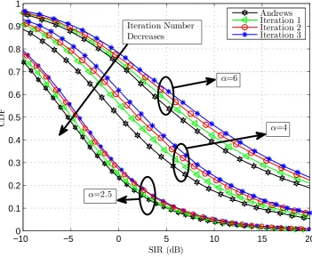
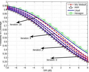
compares the PPP base station model to our proposed Lloyd algorithm model for differentαand iteration values. In these plots,αvalues are 2.5, 4 and 6. The cumulative distribution function (CDF) vs signal-to-interference ratio (SIR) values are plotted for benchmark paper [1] and our proposed approach. One of the common observation in eachαvalue is that PPP deployment provides the lower bound. Also,αplays crucial role in terms having better SIR and coverage as expected. One can easily see that whenαtakes greater values i.e., 4,6, the coverage probability is increasing since greaterα means better received power. In Fig.6, we compare the coverage probability of the random PPP BS/AP model, hexagonal BS/AP model, and Lloyd’s approximation. The tightness of the proposed method for coverage probability is illustrated for different iterations of Lloyd’s algorithm, i.e., {0, 2, 9, 29}. If the iteration value increases then the coverage probability for the proposed method tends to approach the hexagonal BS/AP tessellation. It is important to note that the analytical approximations lose the tractability of Lloyd’s algorithm at larger iteration values such as after iteration number 9. The analytical approximation suffers from the fact that PGFL assumption begins to fail. Nevertheless, the proposed approximation holds for low SIRs.
5. Concluding Remarks
In this study, the impact of Lloyd’s algorithm on the coverage probability of wireless networks is investigated. The link distance distribution is modeled as a mixture of Weibull distributions. Its parameters are derived based on the EM method at each iteration of Lloyd’s algorithm. The numerical results show that if the Lloyd’s algorithm is employed, the transitions between pessimistic PPP to optimistic hexagonal deployment can be approximately modeled.
Conflicts of Interest:“The authors declare no conflict of interest.”
−10 −8 −6 −4 −2 0 2 4 6 8 0.2
0.25 0.3 0.35 0.4 0.45 0.5 0.55 0.6 0.65 0.7 0.75 0.8 0.85 0.9 0.95 1
SIR (dB)
Probability of Coverage
Iteration 0 Iteration 2 Iteration 4 Iteration 9 Iteration 12 Iteration 29 Iteration number
increases
Figure 4.The variation of the coverage probability for a given number of iterations of Lloyd’s algorithm.
−100 −5 0 5 10 15 20
0.1 0.2 0.3 0.4 0.5 0.6 0.7 0.8 0.9 1
SIR (dB)
C
D
F
Andrews Iteration 1 Iteration 2 Iteration 3 Iteration Number
Decreases
α=2.5
α=4 α=6
Figure 5.Proability of coverage for PPP and Lloyd’s algorithm for differentαvalues.
−10 −8 −6 −4 −2 0 2 4 6 8 0.2
0.25 0.3 0.35 0.4 0.45 0.5 0.55 0.6 0.65 0.7 0.75 0.8 0.85 0.9 0.95 1
SIR (dB)
Probability of Coverage
Mix Weibull PPP Lloyd Hexagon
Iteration: 29
Iteration: 2 Iteration: 9
Iteration: 0
Figure 6.The coverage probability for PPP and hexagonal BS/AP deployments and Lloyd’s algorithm
approximation.
MDPI Multidisciplinary Digital Publishing Institute DOAJ Directory of open access journals
TLA Three letter acronym LD linear dichroism
References
1. Andrews, J.G.; Baccelli, F.; Ganti, R.K. A Tractable Approach to Coverage and Rate in Cellular Networks. IEEE Trans. Commun.2011,59, 3122–3134.
2. Heath, R.W.; Kountouris, M.; Bai, T. Modeling Heterogeneous Network Interference Using Poisson Point Processes. IEEE Trans. Signal Process2013,61, 4114–4126.
3. Wu, L.; Zhong, Y.; Zhang, W. Spatial Statistical Modeling for Heterogeneous Cellular Networks - An Empirical Study. Proc. IEEE Veh. Technol. Conf. (VTC); , 2014.
4. Guo, A.; Haenggi, M. Spatial Stochastic Models and Metrics for the Structure of Base Stations in Cellular Networks. IEEE Trans. Wireless Commun.2013,12, 5800–5812.
5. Nakata, I.; Miyoshi, N. Spatial stochastic models for analysis of heterogeneous cellular networks with repulsively deployed base stations.Elsevier Performance Evaluation2014,78, 7–17.
6. Deng, N.; Zhou, W.; Haenggi, M. The Ginibre Point Process as a Model for Wireless Networks with Repulsion. IEEE Trans. Wireless Commun.2014,PP, PP.
7. Okabe, A.; Boots, B.; Sugihara, K.; Chiu, S.N.Spatial Tessellations: Concepts and Applications of Voronoi Diagrams; Wiley: United Kingdom, Jul. 2000.
8. Wang, Z.; Schoenen, R.; Yanikomeroglu, H.; St-Hilaire, M. The Impact of User Spatial Heterogeneity in Heterogeneous Cellular Networks. Proc. IEEE Global Commun. Conf. (GLOBECOM); , 2014.
9. Lloyd, S.P. Least Squares Quantization in PCM.IEEE Trans. Inf. Theory1982,28, 129–137. 10. Newman, D.J. The Hexagon Theorem. IEEE Trans. Inf. Theory1982,28, 137–139.
12. Dempster, A.; Laird, N.; Rubin, D. Maximum likelihood from incomplete data via the EM algorithm. Royal Statistical Society1977,39, 1–38.
13. Nocedal, J. Updating Quasi-Newton Matrices With Limited Storage. Mathematics of Computation1980, 35, 773–782.