Least Upper Delay Bound for VBR Flows in Networks-on- Chip with Virtual Channels

A

Least Upper Delay Bound for VBR Flows in Networks-on-Chip with

Virtual Channels

FAHIMEH JAFARI, KTH Royal Institute of Technology, Sweden ZHONGHAI LU, KTH Royal Institute of Technology, Sweden AXEL JANTSCH, Vienna University of Technology, Austria

Real-time applications such as multimedia and gaming require stringent performance guarantees, usu-ally enforced by a tight upper bound on the maximum end-to-end delay. For FIFO multiplexed on-chip packet switched networks we consider worst-case delay bounds forVariable Bit-Rate (VBR)flows with aggregate scheduling, which schedules multiple flows as an aggregate flow. VBR Flows are characterized by a max-imum transfer size (L), peak rate (p), burstiness(σ), and average sustainable rate(ρ). Based on network calculus, we present and prove theorems to derive per-flow end-to-endEquivalent Service Curves (ESC) which are in turn used for computingLeast Upper Delay Bounds (LUDBs)of individual flows. In a realistic case study we find that the end-to-end delay bound is up to46.9%more accurate than the case without considering the traffic peak behavior. Likewise, results also show similar improvements for synthetic traf-fic patterns. The proposed methodology is implemented in C++ and has low run-time complexity, enabling quick evaluation for large and complex SoCs.

Categories and Subject Descriptors: C.4 [Performance of Systems]: Modeling techniques

General Terms: Design, Performance

Additional Key Words and Phrases: Network-on-chip (NoC), performance evaluation, network calculus, worst-case delay bound, FIFO multiplexing

ACM Reference Format:

Jafari, F., Lu, Z., and Jantsch, A. 2015. Least Upper Delay Bound for VBR Flows in Networks-on-Chip with Virtual Channels. ACM Trans. Des. Autom. Electron. Syst. V, N, Article A (January YYYY), 34 pages. DOI=10.1145/0000000.0000000 http://doi.acm.org/10.1145/0000000.0000000

1. INTRODUCTION

In networks-on-chip, resources like wires, buffers, and switches are shared among multiple communication flows to provide cost efficiency. At the same time many ap-plications have real-time requirements and, consequently, delay and throughput con-straints on the communication. To guarantee maximum delay and minimum through-put for one given communication flow, the interference in the shared resources from other flows has to be analyzed and bounded. We assume that all traffic can be well characterized as flows and scheduled as aggregate which means multiple flows are scheduled as an aggregate flow. For a given flow, we study the maximum interference of all other flows based on the network calculus theory [Le Boudec et al. 2004].

Author’s addresses: F. Jafari and Z. Lu, Department of Electronic and Computer Systems, School of Information and Communication Technology, KTH Royal Institute of Technology, Stockholm, Sweden; email: {fjafari, zhonghai}@kth.se; A. Jantsch, Vienna University of Technology, Vienna, Austria; email: [email protected].

Permission to make digital or hard copies of part or all of this work for personal or classroom use is granted without fee provided that copies are not made or distributed for profit or commercial advantage and that copies show this notice on the first page or initial screen of a display along with the full citation. Copyrights for components of this work owned by others than ACM must be honored. Abstracting with credit is per-mitted. To copy otherwise, to republish, to post on servers, to redistribute to lists, or to use any component of this work in other works requires prior specific permission and/or a fee. Permissions may be requested from Publications Dept., ACM, Inc., 2 Penn Plaza, Suite 701, New York, NY 10121-0701 USA, fax+1 (212) 869-0481, or [email protected].

c

YYYY ACM 1084-4309/YYYY/01-ARTA $10.00

In network calculus, flows are characterized asarrival curvesand the service offered to flows by a network element such as a link or a switch is abstracted asservice curve. Since the network contention for shared resources includes not only direct contention but also indirect contention, predicting the worst-case performance is extremely hard. To calculate the accurate delay bound per flow, the main problem is to obtain the end-to-end Equivalent Service Curve (ESC) and internal output arrival curves of individ-ual flows in an arbitrary network of servers in terms of the latencies of the individindivid-ual schedulers in the network. Since the required theorems for calculating performance metrics of VBR traffic transmitted in the FIFO order and scheduled as aggregate have not been represented so far, we [Jafari et al. 2011; Jafari et al. 2012] have defined and proved them based on network calculus [Chang 2000; Le Boudec et al. 2004]. In [Ja-fari et al. 2011], we proposed and proved the required theorem for deriving the output characterization of VBR traffic under the defined system model to have exact vision about output metrics used for obtaining performance bounds. In [Jafari et al. 2012], the required theorems for computing end-to-end ESC and end-to-end delay bound are defined and proved. Moreover, we presented a simple example to show how the pro-posed theorems can be used in the network. The method presented in [Jafari et al. 2012] only considers direct contentions of a tagged flow. In this paper, we use the pro-posed theorems [Jafari et al. 2011; Jafari et al. 2012] to present a formal approach for performance analysis modeling both direct and indirect contentions.

VBR is a class of traffic in which the rate can vary significantly from time to time, containing bursts. Real-time compressed voice and video and time-sensitive bursty data traffic are examples of VBR traffic. Real-time VBR flows can be characterized by a set of four parameters,(L, p, σ, ρ), whereLis the maximum transfer size,ppeak rate, σburstiness, andρaverage sustainable rate [Le Boudec et al. 2004]. For instance, in a NoC with a link data width of32bits, frequency of500MHz. This means a link band-width of16Gbits/s (32bits×500MHz). An HDTV video stream can be characterized with L = 32bits, p = 16Gbits/s, σ = 960Kbits, ρ = 76Mbits/s. Our assumption is that the application-specific nature of the network enables to characterize traffic with sufficient accuracy.

For an individual flow, called atagged flow, we first consider resource sharing sce-narios (channel sharing, buffer sharing, and channel&buffer sharing) in the routers and then build analysis models for different resource sharing components. We assume that the routers employ round robin scheduling to share the link bandwidth. Based on these models, we can derive the intra-router ESC for an individual flow. To con-sider the contention which a flow may experience along its routing path, we present a recursive algorithm to classify and analyze flow interference patterns. The algorithm uses the proposed theorems to analyze the effect of contention flows on the tagged flow. Based on this algorithm, we derive the end-to-end ESC and then Least Upper Delay Bound (LUDB) for a tagged flow under the mentioned system model. To show the po-tential of our method, we experiment three case studies to derive delay bounds and compare them with simulation results. It is worth mentioning that the paper does not deal with the back-pressure, but calculates the buffer size thresholds to make sure the back-pressure does not occur in the network.

Least Upper Delay Bound for VBR Flows in Networks-on-Chip with Virtual Channels1 A:3

2. RELATED WORK

Recently, NoC designers have a great deal of interest in the development of analytical performance models [Bakhouya et al. 2011]. Ogras et al. [2005 ] give a unified rep-resentation of NoC architectures and applications and consider some major research problems in the design area. As represented in this work, most of research problems need to analytically analyze and evaluate performance metrics in the network. we [Kiasari et al. 2013] have surveyed four popular mathematical formalisms -dataflow analysis, schedulability analysis, queueing theory, and network calculus- along with their applications in NoCs. Also, we have reviewed strengths and weaknesses of each technique and its suitability for a specific purpose.

Dataflow analysisis a deterministic approach based on graph theory. As an example, Hansson et al. [2008 ] present a model using a cyclo-static dataflow graph for buffer dimensioning for NoC applications. In dataflow analysis, it is assumed that the pat-tern of communication among cores and switches are deterministic and predefined. Dataflow analysis must be used with restricted models such as DDF and CSDF to capture dynamic behavior. In other words, the expressiveness is typically traded off against analyzability and implementation efficiency in this formalism.

Schedulability analysisis an analytical approach for investigating the timing prop-erties in real-time systems. It gets a set of tasks, their worst-case execution time, and a scheduling policy as inputs and determines whether these tasks can be scheduled such that deadline misses never occur. One example of this approach in NoCs is pre-sented by Shi and Burns [2008 ]. Schedulability analysis uses simpler event models compared to the other mathematical formalisms and consequently the performance model is easily extracted with less accuracy.

The proposed models by Lee [2003 ] and Rahmati et al. [2009 ; 2013 ] are inspired by schedulability analysis. Lee [2003 ] presents a worst-case analysis model for real-time communication and also proposes a feasibility test algorithm for a simplex virtual circuit in wormhole networks. This work is extended by Rahmati et al. [2009 ] towards NoCs, computing real-time bounds for high bandwidth traffic. They also extend the model [2013 ] to provide more detailed switch models and consider virtual channels and variable buffer lengths. The key advantage of these methods is that they compute the worst-case bounds with low time complexity without any special hardware support, but the main limitation is that they do not leverage the input arrival patterns, which it leads to over approximations of the performance analysis.

can account for nonstationary observed in packet arrival processes. They also investi-gated the impact of packet injection rate and the data packet sizes on the multifractal spectrum of NoC traffic.

Network calculus is a mathematical framework for deriving worst-case bounds on maximum latency, backlog, and minimum throughput in network-based systems. It is able to model all traffic patterns with bounds defined by arrival curves. In this respect, designers can capture some dynamic features of the network based on shapes of the traffic flows [Bakhouya et al. 2011]. Network calculus can also abstract many schedul-ing algorithms and arrival classes at sschedul-ingle queue with multiplexed arrival flows, by service curves. The service curves through a network can be convolved as a single ser-vice curve. Hence a multi-node network analysis can be simplified to a single-node analysis. Regarding these two features, network calculus can analyze many schedul-ing algorithms and arrival classes over a multi-node network in a uniform framework while classical queuing theory separately models different combination of them [Ciucu et al. 2012]. The probabilistic version of (deterministic) network calculus is stochastic network calculus. In some networks, such as wireless networks, the service offered by a communication channel may vary randomly over time due to channel contention and impairment. Such networks can only provide stochastic services and guarantees. For example, Rizk and Fidler [2012 ] use stochastic network calculus to derive per-flow end-to-end performance bounds in a network of tandem queues under open-loop fBm cross traffic which is a model for self-similar and long-range dependent aggregate In-ternet traffic. Since we employ deterministic network calculus, in the rest of our paper, network calculus refers to the deterministic type. A network calculus-based methodol-ogy [Bakhouya et al. 2011] analyzes and evaluates performance and cost metrics, such as latency, energy consumption, and area requirements in on-chip interconnects. Au-thors in this paper compare 2D mesh, spidergon, and WK-recursive topologies using a given traffic pattern and show that WK-recursive outperforms mesh and spidergon in all considered metrics. The proposed model in this paper is simple without consid-ering virtual channel effects and modeling all interferences between flows sharing a resource in the network. Moreover, the model does not investigate the peak behavior of flows which leads to less accurate bounds while we consider performance analysis for VBR traffic in on-chip networks employing aggregate resource management.

The performance evaluation of real-time services in networks employing aggregate scheduling is particularly challenging because of its complexity. Aggregate scheduling arises in many cases. In addition to NoC, for example, it can also be applied for ob-taining scalability in large-size networks. The Differentiated Service (DiffServ) [Blake et al. 1998] is an example of an architecture based on aggregate scheduling in the Internet. Despite the research efforts, few results have appeared on this subject. A survey on the subject can be found in [Bennett et al. 2002]. Charny et al. [2000 ] con-sider a closed-form delay bound for a generic network configuration under the fluid model assumption. It is also extended by Jiang [2002 ] to consider packetization ef-fects. However, these works can derive bounds only for small utilization factors in a generic network configuration.

Least Upper Delay Bound for VBR Flows in Networks-on-Chip with Virtual Channels1 A:5

The computation of delay bounds through network calculus in feed-forward net-works under arbitrary multiplexing has already been addressed in different lectures [Schmitt et al. 2008; Kiefer et al. 2010; Bouillard et al. 2010]. One of these works [Bouillard et al. 2010] describes the first algorithm which can compute the worst-case end-to-end delay for a given flow for any feed-forward network under blind multiplex-ing, with concave arrival curves and convex service curves. Since the problem is in-trinsically difficult (NP-hard), the authors show that in some cases, like tandem net-works with cross-traffic interfering along intervals of servers, the complexity becomes polynomial. Then, the approach is refined [Bouillard et al. 2011] in order to take into account fixed priorities. Bouillard et al. study networks with a fixed priority service policy which means each flow is assigned a fixed priority and try to take into account the pay multiplexing only once (PMOO) phenomenon. This stream of works deal with networks of arbitrary multiplexing also known as general or blind multiplexing, which means no assumption is made about the service policy while by assuming an explicit multiplexing scheme like FIFO, tighter bounds can be obtained.

A related stream of works [Lenzini et al. 2006; Lenzini et al. 2008; Bisti et al. 2010] propose a methodology which calculates delay bounds in tandem networks of rate-latency nodes traversed by leaky bucket shaped flows. They also introduce a software tool, called DEBORAH, which implements algorithms employed in their methodology to compute delay bounds. These works consider servers in tandem or sink trees, while our proposed method computes end-to-end delay in a generic topology of NoC. More-over, these works investigate computing delay bounds only for average behavior of flows and they do not consider peak behavior, which results in less accurate bounds.

Boyer [2010 ] tries to model shaping for an end-to-end delay where each server is shared by two flows. An applicative token bucketγr,b is shaped by the bit-rate of the

linkλR, leading to a two-slopes affine arrival curve which this arrival curve is similar

to one we consider for double leaky buckets. The paper investigates a simple topology, a sequence of rate-latency servers, each one shared by two flows with a FIFO policy, and a simple case of nested contentions. Moreover, authors state that their model-ing is incomplete: when computmodel-ing the worst-case traversal time of a flow, they model only the shaping on the considering flow, not on the interfering ones (leading to the title ‘half-modeling of shaping’) In this paper, we investigate both nested and crossed contentions in general to model all flows (even interfering ones) with complex interfer-ences in on-chip networks.

All aforementioned works in the subject of aggregate resource management compute delay bounds in various network infrastructures but not on-chip networks. As regards to NoC architecture, analytical models are very close to the reality of the system. For instance, a router in on-chip networks can be modeled in pure hardware which means the micro-architecture is feasible for analysis. Therefore, network calculus can provide the analysis more accurate in on-chip networks.

Qian et al. [2010 ] present analytical models for traffic flows under strict priority queueing and weighted round robin scheduling in on-chip networks. They then derive per-flow end-to-end delay bounds using these models. Like most of mentioned works, the proposed model by Qian et al. [2010 ] does not deal with peak behavior of flows, which results in less accurate bounds. The proposed method in this paper considers performance analysis for VBR traffic characterized by (L, p, σ, ρ)in on-chip networks employing aggregate resource management. As such, our method achieves more accu-rate delay bounds.

3. NETWORK CALCULUS BACKGROUND

o

lum

e

j jt

σ +ρ

j

σ

data v

o

L

j j

L +p t

j

L

ti

j j j

j j

L

p σ θ

ρ − =

−

time

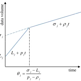
Fig. 1. Arrival curve of flowfjwith TSPEC(Lj, pj, σj, ρj).

(TSPEC) [Wroclawski 1997] to model the average and peak characteristics of flowfjas

arrival curveαj(t) =min(Lj+pjt, σj+ρjt)in whichLj is the maximum transfer size,

pjthe peak rate(pj ≥ρj),σjthe burstiness(σj≥Lj), andρjthe average (sustainable)

rate. We denote it asfj ∝(Lj, pj, σj, ρj). As shown in Figure 1,θj = (σj−Lj)/(pj−ρj)

andαj(t) =Lj+pjtift≤θj;αj(t) =σj+ρjt, otherwise.

In this paper, we also consider a class of curves, namely pseudoaffine curves [Lenzini et al. 2006], which is a multiple affine curve shifted to the right and given by β = δT ⊗[⊗1≤x≤nγσx,ρx]. In fact, a pseudoaffine curve represents the service received by

single flows in tandems of FIFO multiplexing rate-latency nodes. Due to concave affine curves, it can be rewritten asβ =δT ⊗[∧1≤x≤nγσx,ρx], where the non-negative termT

is denoted as offset, and the affine curves between square brackets as leaky-bucket stages. It is clear that a rate-latency service curve is in fact pseudoaffine, since it can be expressed asβ=δT⊗γ0,R.

Given arrival curve αand service curveβ, the delay is bounded by the horizontal deviation between the arrival and service curves.

4. SYSTEM MODEL AND NOTATIONS

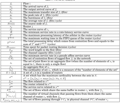
As depicted in Figure 2, we consider an NoC architecture in which every node contains a router and a core which performs its own computational, storage or I/O processing functionality, and is equipped with a Network Interface (NI). As you can see in the fig-ure, buffers are arranged to construct VCs in each input channel. To characterize flows based on their defined TSPEC, we assume unbuffered leaky bucket controllers (regu-lators) which do not buffer the packets, but stall the traffic producers or IPs [Jafari et al. 2010].

Assumptions in this work are listed as follows:

— The NoC architecture can have different topologies.

— Packets have fixed length and traverse the network in a best-effort fashion with virtual-cut-through switching technique using a deadlock-free deterministic routing. — Routers have only input buffers and VCs.

— Buffers are bounded and the network is lossless.

— The router can have multiple VCs per in-port. VC allocation is deterministic and each VC receives an aggregate service.

— All traffic is the part of TSPEC flows f = T SP EC(L, p, σ, ρ) at the entry into the network.

Least Upper Delay Bound for VBR Flows in Networks-on-Chip with Virtual Channels1 A:7

4 r

1

r r2 r3

2

f

1

f

Core

8 r 6

r r₇

5 r

2

f

1

f

5

f

Core Core Core Core

ejection channel injection

channel

Network Interface (NI)

DEMUX

10

r r₁₁

9

r r₁₂

3

f

4

f

2

f

Core

Core Core Core Core

Core CoreCore Core

ou

tp

ut

c

h

a

n

n

e

in

put

chann

e

1 1

q

DE

M

U

X

DE

M

13

r r14 r₁₅ r₁₆

f

5

f f₃

Core

Core Core CoreCore Core

Core Core Core

Crossbar Switch ls

e

ls

p q

Routing Control Unit

M

UX

Arbiter

4

f

Fig. 2. An example of an NoC with16nodes and5flows along with the structure of a single node.

— Flows are classified into a pre-specified number of aggregates.

— Traffic of each aggregate is buffered and transmitted in the FIFO order, denoted as FIFO multiplexing.

— Different aggregates are buffered separately and each aggregate is guaranteed a rate-latency service curve.

— We use a concrete policy, in this case, round-robin arbitration, to support the assump-tion on rate-latency service curve. Indeed, it can use some other arbitraassump-tion policies as well. We also assume a fixed word length ofLwin all of flows.

— The peak rate is limited by the hardware. It is always 1flit/cycle.

NoC designers can obtain per flow end-to-end delay bound in NoC architectures by the proposed method in this paper under the mentioned assumptions.

Most of assumptions in this paper have been widely used by some previous models [Qian et al. 2009; Jafari et al. 2010]. The system model in this paper is more general than the mentioned models [Qian et al. 2009; Jafari et al. 2010] because they consider a Constant Bit Rate (CBR) flow in NoCs, defined by (σ, ρ) which is a special case of TSPEC. Furthermore, we have relaxed a significant limitation of the previous analyt-ical model [Jafari et al. 2010] which presumes the number of VCs for each PC is the same as the number of flows passing through that channel.

We use an example depicted in Figure 2 to explain terminology used in the paper. The figure shows a network with16nodes numbered from1,2, ...,16connected by links. There are 5flows in the example denoted as f1, ..., f5. Multiple flows share the same

buffer and channel in the router are scheduled as a flow called aggregate flow. For instance,f{1,2} in router3is an aggregate flow. Atagged flowis the flow that we shall derive its delay bound and other flows that share resources with the tagged flow are contention flows. In this example,f1is the tagged flow, andf2,f3, andf4are contention

flows. Notations in the paper are listed in Table I.

We use sub-index ”(fi, rj)” for notations to indicate that they are related to flowfiin

routerrj. For example,α(f1,r2)denotes the arrival curve of flowf1in routerr2. We also employ sub-index ”(si, rj)” to state notations are related tofsiin routerrj. In this case,

Table I. The list of notations

fi Flowi

αi The arrival curve offi

α∗_i The output arrival curve offi

Li The maximum transfer size offi(flits)

pi The peak rate offi(flits/cycle)

σi The burstiness offi(flits)

ρi The average rate offi(flits/cycle)

Src(i) The source node offi

rj Routerj

βj The service curve ofrj

R The minimum service rate in a rate-latency service curve

Tl _{The maximum processing latency of the arbiter in the router(cycles)}

THoL _{The maximum waiting time in the FIFO queue of the router(cycles)}

TT otal The total processing delay which comes from contention flows and equals to the

sum ofTl_andTHoL_(cycles)

Drouter Time spent for packet routing decision(cycles)

Lw The word length in the flow(flits)

C The channel capacity(flits/cycle)

ρx The minimum service rate in a pseudo affine service curve

CFt The set of contention flows of tagged flowftin the network

si The set of joint flows in an aggregate flow (when the number of elements of_{equal to1, there is only a single flow)} siis

fsi An aggregate flow ofsi

|si| The cardinality of setsi, which is a measure of the ”number of elements of the set”

S={si} A set ofsi’s in a tandem of routers

sm A set which has the maximum cardinality between the sets inS.

sm₌ sx

|sx|=max(|si|) ;∀si∈S

fsm The flow related tosm

rm _{The router related tos}m

βm _{The service curve related tos}m

FB

(si,rj) The set of flows which share the same buffer in routerrjwith flowfsi

V(si,rj)

The number of virtual channels that passing flows from them share the same channel of routerrjwith flowfsi

F_{(V C}

k,P Ci,rj) The set of flows passing throughV Ckin physical channelP Ciof routerrj

5. PROPOSED THEOREMS

In this section, we review the earlier proposed theorems [Jafari et al. 2011; Jafari et al. 2012] which are required for analyzing performance of VBR flows in a FIFO multiplexing network.

We first represent a theorem for computing delay bound as follows.

Theorem 1. (Delay Bound) Letβ be a pseudo affine curve, with offsetT andn

leaky-bucket stageγσx,ρx, 1≤x≤n, this means we have:

β=δT⊗[⊗1≤x≤nγσx,ρx] =δT ⊗[∧1≤x≤nγσx,ρx]

and let α = min(L+pt, σ+ρt) = γL,p∧γσ,ρ. Ifρ∗β ≥ ρ(ρ

∗

β = min1≤x≤nρx), then the

maximum delay for the flow is bounded by

h(α, β) =T+

"

∨1≤x≤n

L−σx+θ(p−ρx) +

ρx

#+

(1)

Least Upper Delay Bound for VBR Flows in Networks-on-Chip with Virtual Channels1 A:9

In the rest of the paper, we apply Theorem 1 on the end-to-end ESC to calculate LUDB for a tagged flow. Due to our proposed method in Section 6, to obtain the end-to-end ESC, we should able to subtract contention flows from a service curve. To this end, we propose Proposition 1 and Theorem 2. In Proposition 1, we derive ESC with FIFO multiplexing where service curve is a pseudo affine curve. We then use Corollary 1 which is an immediate consequence of Proposition 1 to propose Theorem 2. This theorem is employed for deriving ESC in the underlying system model.

In Proposition 1 and Theorem 2, we obtain ESC with FIFO multiplexing under dif-ferent assumptions.

Proposition 1. (Equivalent Service Curve) Letβ be a pseudo affine curve, with offset

T andnleaky-bucket stageγσx,ρx, 1≤x≤n, this means we have:

β=δT ⊗[⊗1≤x≤nγσx,ρx] =δT⊗[∧1≤x≤nγσx,ρx]

and let α = min(L +pt, σ +ρt) = γL,p∧ γσ,ρ. If ρ∗β ≥ ρ (ρ

∗

β = min1≤x≤nρx) and

p ≥ ρ◦_β (ρ◦_β = max1≤x≤nρx), then the ESC obtained by subtracting arrival curve α, {βeq_{(α, τ), τ=h(α, β)} ≡β}eq_{(α), with}

βeq(α) =δ

T+∨1≤i≤n

h_{L−σi+θ(p−ρi)+}

ρi

i+

+θ⊗[⊗1≤x≤n[

γ

ρx

∨1≤i≤n

h_{L−σi+θ(p−ρi)+}

ρi

i+

−σ−σx−_ρx(ρx−ρ)θ

,ρx−ρ

## ₍₂₎

PROOF. We have proved it in [Jafari et al. 2012]. See Appendix B.

The following corollary is an immediate consequence.

Corollary 1. Letβ=δT ⊗γσx,ρxbe a pseudo affine curve, with offsetT and one

leaky-bucket stageγσx,ρx, and letα=min(L+pt, σ+ρt) =γL,p∧γσ,ρ. Ifρx≥ρandp≥ρx, then the ESC obtained by subtracting arrival curveα,βeq

βeq =δ

T+hL−σx+θ(p−ρx)+ ρx

i+

+θ⊗γ0,ρx−ρ (3)

PROOF. We can easily obtain this corollary by applying Proposition 1 for service curveβ whenn= 1.

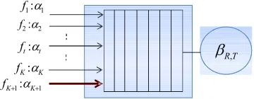
We can specifically capitalize on Corollary 1 to obtain a parametric expression for the ESC of a tagged flow passing through a rate-latency node. We assume the number of flows passing through this node isK+1. Therefore, for computing equivalent service curve for the tagged flow, we should subtract the arrival curves of otherKflows. It can be calculated by iteratively applying Corollary 1 forKtimes. Without loss of generality, we presume that the tagged flow is flowK+ 1. We now present following theorem:

Theorem 2. (Equivalent Service Curve for Rate-Latency Service Curve with K+ 1

Flows) Consider one node with a rate-latency service curveβR,T =δT ⊗γ0,R. Letαi =

min(Li+pit, σi+ρit) =γLi,pi∧γσi,ρibe arrival curve of flowiandpi≥R− PK+1

(j=1;j6=i)ρj,

T

R,

b

1:a

f

K K f :a

1 1: +

+ K

K

f a

t t f:a

2 2:a

f

Fig. 3. Computation of equivalent service curve for flowK+ 1in a rate-latency node.

shown in Figure 3. Assuming PK+1

j=1 ρj ≤ link rate, whereC is the link rate, the ESC

for flowK+ 1in the node, obtained by subtractingKarrival curves, is:

βeq_K+1=δ

T+PK i=1

"

Li+θi(pi−R+Pi−1

j=1ρj)+

R−Pi−1

j=1ρj

#+

+θi

!⊗γ_0,R−PK

j=1ρj ₍₄₎

PROOF. We have proved it in [Jafari et al. 2012]. See Appendix C.

Theorem 3 states how output arrival curve of a VBR flow in a FIFO multiplexing node can be calculated.

Theorem 3. (Output Arrival Curve with FIFO) Consider a VBR flow, with TSPEC

(L, p, ρ, σ), served in a node that guarantees to the flow a pseudo affine service curve

β =δT ⊗γσx,ρx. The output arrival curveα

∗_{given by:}

α∗=

 



θ > T γ(p∧ρx)T+θ(p−ρx)++L−σx,p∧ρx ∧γσ−σx+ρT ,ρ

θ≤T γσ−σx+ρT ,ρ

(5)

PROOF. We have proved it in [Jafari et al. 2011]. See Appendix D.

We apply this theorem to calculate internal output arrival curves. For instance, in Section 6.2, we obtain the output arrival curve of a crossed flow when it is split into two nested flows.

6. FORMAL METHOD FOR LUDB DERIVATION

We have presented and proved the required theorems for deriving LUDB for VBR flows in on-chip networks based on aggregate scheduling with multiple virtual channels. As mentioned before, to calculate LUDB per flow, we should first obtain the end-to-end ESC which the tandem of routers provides to the flow. For calculating the end-to-end ESC, we propose two following steps:

•Step 1:Intra-router ESC

•Step 2:Inter-router ESC

Least Upper Delay Bound for VBR Flows in Networks-on-Chip with Virtual Channels1 A:11 Crossbar Switch D E M U X Channel 2 f 1 f

Ø

Buffer&Channel Sharing

• Set of contention flows of tagged flow , sharing both buffer and channel in router

denoted as CB

r fi j

F_{( , )} i

f rj

Crossbar Switch D E M U X Channel

{ }1,2

f

• We consider them as an aggregated flow and calculate inter-router ESC for the aggregated flow

Fig. 4. An example of channel&buffer sharing.

Crossbar Switch D E M U X Channel 3 f 1 f DEMUX C L F F C r f w C j r i f C j r i f j

i _÷´

ø ö ç è æ -Ä = 1 , 0 ) , ( ) , ( ) , (

d

g

b

= ; ( , ) 1

) , ( ) , ( ) , (

• If

f

is the tagged flow:

C L T C

R P w

r f r

f,)= ( ,)=

(1 ₂; 1

• In the example

f

is the tagged flow and we have

Ø

Channel Sharing

• Set of contention flows of tagged flow , sharing a channel in router denoted as C

j r i f

F_{( , )} i f j r 2 f

Fig. 5. An example of a channel sharing three flows.

6.1. Step1: Intra-router ESC

To compute intra-router ESC for a tagged flow, it is necessary to investigate resource sharing. At each router, we identify three types of resource sharing, namely, chan-nel sharing,buffer sharing, andchannel&buffer sharing.Channel sharingmeans that multiple flows share the same out-port and thus the output channel bandwidth.Buffer sharing means that multiple flows share the same buffer but not channel. In chan-nel&buffer sharing, multiple flows share both buffers and channels. They are sched-uled as a flow called aggregate flow.

6.1.1. Channel&Buffer Sharing.Figure 4 depicts an example of flows sharing both chan-nel and buffer in the router. As shown in the figure, we consider these flows as an aggregate flow. When an aggregate flow includes the tagged flow, it is called astagged aggregate flow. In this respect, we calculate intra-router ESC for the tagged aggregate flow in the router instead of the tagged flow. In Section 6.2, we show how ESC of the tagged flow is extracted from the ESC of the tagged aggregate flow by removing con-tention flows one by one. For simplicity, in the rest of the paper, ”tagged flow” refers to both tagged flow and tagged aggregate flow.

6.1.2. Channel Sharing.Figure 5 depicts a channel shared between three flows f1,f2,

and f3. Since the arbitration policy determines how much the flows influence each

other, it has to be known. We assume that, while serving multiple flows, the routers employ round robin scheduling to share the channel bandwidth. Assuming a fixed word length ofLwin all of flows, round robin arbitration means that each flowfsi in router

rj gets at least a C V(si,rj)

of the channel bandwidth, whereC is the channel capacity

and V(si,rj)

the number of virtual channels that passing flows from them share the same channel of router rj with flowfsi. A flow may get more if other flows use less,

but we now know a worst-case lower bound on the bandwidth. Round robin arbitration has good isolation properties because the minimum bandwidth for each flow does not depend on properties of the other flows.

Crossbar D E M U X Channel 1 f 2 f P2 P2 P2 P2 ... P2 P2 P1 1 f 0 ) , ( ) , ( 1 1 = = P r f r f T C R Crossbar Switch C h a n n e l 2 f 0 ) , ( ) , ( 2 2 = = P r f r f T C R

Fig. 6. An example of a buffer sharing two flows.

robin arbiter in routerrj for flowfsi as a rate-latency server [Gebali et al. 2009] that

its function is asβ(si,rj)=R(si,rj)(t−T l (si,rj))

+_{, whereR}

(si,rj)is the minimum service

rate andTl

(si,rj)is the maximum processing latency of the arbiter in routerrjfor flow

fsi.R(si,rj)andT l

(si,rj)are defined as follows:

R(si,rj)=

C

V(si,rj)

(6)

T_(sl_i,rj)= V(si,rj) −1 × _L w

C +Drouter

(7)

whereDrouteris the delay for packet routing decision in a router.

As mentioned in Section 5, a rate-latency service curve is in fact a pseudoaffine. Therefore,β(si,rj)can be expressed asδ

V(si,rj) −1

×(Lw

C +Drouter)⊗

γ_0, C

V(si,rj)

. Assuming

f1is the tagged flow in the example,β(f1,r)=δ2×(Lw

C +Drouter)⊗γ0,C3.

6.1.3. Buffer Sharing. Figure 6 shows a buffer shared between two flowsf1 andf2. In

this type of sharing, in addition to maximum processing latency for link sharing, Tl_,

we introduce the head-of-Line delay for a tagged flow as below:

Head-of-Line delay (HoL): Given a flow comes at timet in a router, the maximum waiting time in the FIFO queue would be in timet+THoL_.

Therefore, the total processing delay which comes from contention flows for tagged flowfsiin routerrj,T

T otal

(si,rj), is equal toT

l_+THoL

We assumef1in Figure 6 is the tagged flow. According to Equation (7),T_(fl

1,r)= 0. From the figure, it is clear that T_(fHoL

1,r) is equal to the maximum delay for passing packets of flowf2in the buffer. According to the network calculus theory [Le Boudec

et al. 2004], the maximum delay for flowfj is bounded by Equation (8).

¯

D(fj,r)=T l (fj,r)+

Lj+θj(pj−R(fj,r)) +

R(fj, r)

(8)

Therefore, we formulateTHoL

(f1,r)as follows:

T_(fHoL_1,r)=T_(fl_2,r)−θ2+

L2+θ2p2

R(f2,r)

Least Upper Delay Bound for VBR Flows in Networks-on-Chip with Virtual Channels1 A:13

P2

P3

P3

P₂

...

P3

P2

P1

1

f

3

f

Crossbar

D

E

M

U

X

Channel

1

f

2

f

3

f

2

f

C

h

a

n

n

e

l

3

f

Crossbar Switch

C

h

a

n

n

e

l

Fig. 7. An example of a buffer sharing three flows.

If there is more than one flow sharing the buffer with the tagged flow as shown in Figure 7, HoL delay for tagged flowfsiin routerrjis given by

T_(sHoL

i,rj)= X

∀fc∈F₍B_si,rj)

THoL(fc)

(si,rj) (10)

whereFB

(si,rj)is the set of flows which share the same buffer in routerrjwith tagged

flowfsi.T HoL(fc)

(si,rj) is calculated as follows.

THoL(fc) (si,rj) =T

l

(fc,r)−θc+

Lc+θcpc

R(fc,r)

(11)

Therefore routerrj can serve flow fsi by curve β(si,rj) = δTT otal

(si,rj) ⊗γ0,R(si,rj), where TT otal

(si,rj)=T HoL (si,rj)+T

l

(si,rj)andR(si,rj)is calculated by Equation (6).

We analyze the buffer space threshold for each VC based on traffic specifications of flows passing through that VC, and also interference between them. The buffer space threshold for virtual channel V Ck in physical channel P Ci of router rj is given as

below:

B(V Ck,P Ci,rj)=

X

∀fc∈F(V Ck,P Ci,rj)

σc+ρcT_(fp c,rj)+

θ−T_(fp

c,rj) +h

pc−R(fc,rj) +

−pc+ρc

i

(12)

whereF(V Ck,P Ci,rj)is the set of flows passing throughV Ckin physical channelP Ci

of routerrj.

6.2. Step2: Inter-router ESC

analysis model which keeps only channel&buffer sharing for tagged flow. This model is calledaggregate analysis model. For example, suppose that a tagged flowf1traverses

a tandem of routers, and is multiplexed with contention flows as depicted in Figure 8(a). After analyzing intra-router ESC, aggregate analysis model is shown as 8(b). In this model, β(si,rj) indicates that the service curve is related to flowfsi in router rj.

For instance,β({1,2},r3)is the service curve of flowf{1,2}in routerr3.f{1,2}indicates to a flow aggregated by flowsf1andf2. A set ofsi’s in a tandem of routers is denoted as

S ={si}. For example, in Figure 8(b),S={{1},{1,2,3},{1,2},{1}}.

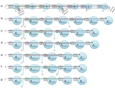
Now, we consider aggregate analysis model to recognize interference patterns and remove contention flows one by one. A tagged flow directly contends with contention flows. Also, contention flows may contend with each other and then contend with the tagged flow again. To consider inter-ESC in the aggregate analysis model, we decom-pose a complex contention scenario to two basic contention patterns, namely, Nested and Crossed.Figures 8, 9, 10, and 11 illustrate examples of different kinds of nested contentions and an example of crossed contention is shown in Figure 12. In the follow-ing, we will describe these examples with more details.

We use the algebra of sets to recognize the contention scenarios. To facilitate our discussion, we define convenient notations by the example in Figure 8(b). In the ex-ample, the tandem of servers is as

β({1},r1), β({1,2,3},r2), β({1,2},r3), β({1},r4) and S =

{si} ={{1},{1,2,3},{1,2},{1}}. We definesm=

sx

|sx|=max(|si|) ;∀si∈S , where |sx|is the cardinality (the number of elements) of setsx. The service curve, flow, and

router related tosm_{are denoted asf}

sm,βm, andrm, respectively. Thus, in Figure 8(b),

sm_={1,2,3},f

sm=f_{1,2,3},rm=r₂, andβm=β_({1,2,3},r

2).

We denote the service curve placed before βm on the aggregate analysis model by βP rev_{and related aggregate flow and router asf}

sP rev andrP rev, respectively. Notation

βN extindicates to the service curve placed after βm, as well. Therefore, due toβm = β({1,2,3},r2) in Figure 8(b), β

P rev _{= β}

({1},r1), s

P rev _{= {1}, f}

sP rev = f_{1}, rP rev = r1,

βN ext_=β

({1,2},r3),s

N ext_={1,2},f

sN ext =f_{1,2},rN ext=r3.

Contention recognition procedure in an aggregate analysis model can be generalized as following steps:

(1) Findsm₌

sx

|sx|=max(|si|) ;∀si∈S .

(2) ifsP rev_⊂sN ext_{then the contention isNested; –Removef}

sm_−(sm_∩sP rev₎fromβm.

(3) ifsN ext_⊂sP rev_{then the contention isNested; –Removef}

sm_−(sm_∩sN ext₎fromβm

(4) else

(a) ifsP rev_⊂sm_andsN ext_6⊂sm_{then the contention isNested;}

— Removefsm_−(sm_∩sP rev₎fromβm.

(b) ifsN ext⊂smandsP rev6⊂smthen the contention isNested; — Removefsm_−(sm_∩sN ext₎fromβm

(c) else, it isCrossed.

— The problem is strictly transformed to the combination of two nested flows

To remove a contention flow from a service curve and derive the new service curve from that, we apply the proposed corollary 1 in Section 5.

When sm_{is not unique, each of them can be selected. In this paper, we choose the}

first one from the left side in the aggregate analysis network. In the case ofsN ext_=sP rev_{, there are two possibilities:}

Least Upper Delay Bound for VBR Flows in Networks-on-Chip with Virtual Channels1 A:15

Nested Flows-Case 1

1

f

a)

1

r r2 r3 r₄

2

f f3

b)

c)

{1,2,3},) ( r2

β 1

f

2

f f3

{ }1,2, ) ( r3

β

1

f

2

f

{ }1,2, ) ( r3

β

{ }1, ) ( r1

β β({ }1,r4)

{ }1, ) ( r1

β β({ }1,2,r2) β({ }1,r4)

Fig. 8. Analysis for the first type of nested flows.

1 f 3 f 2 f a) 1

r

r

r

r

Nested Flows-Case 2

1

f

2

f f3

{ }1, ) ( r4

β

1

f

2

f

{ }1, ) ( r4

β

b)

c)

{ }1, ) ( r1

β

{ }1, ) ( r1

β β({ }1,2,r2) { }1,2, ) ( r2

β _{({1,2,3}, )}

3

r

β

{ }1,2, ) ( r3

β

Fig. 9. Analysis for the second type of nested flows.

1 f 3 f a) 1

r r₂ r3 r4 r5

4 f Nested Flows-Case 3

2

f

1

f

2

f f3

{ }1,4, )

( r4

β 1 f 2 f b) c)

{ }1,)

( r1

β

{ }1,)

( r1

β β({ }1,2,r2)

{ }1,2, )

( r2

β β({1,2,3},r3)

{ }1,2, )

( r3

β

4 f

{ }1, )

( r5

β

{ }1,4, )

( r4

β

4 f

{ }1, )

( r5

β

Fig. 10. Analysis for the third type of nested flows.

(2) sN ext =sP rev = sm: In this case, three nodessN ext, sP rev, and smshould be com-bined as a single server by applying the theorem ofconcatenation of network ele-ments[Le Boudec et al. 2004]. It will be discussed in Section 6.3.

In the following, we give examples for various contention patterns.

6.2.1. Nested Flows.Four different types of nested contention are exemplified as Fig-ures 8, 9, 10, and 11. Flowf3is nested in flowf2in Figures 8, 9, and 10 and it is also

1 f 2 f a) 3

r r4 r5

2 r 1 r 3 f 4 f 1 f 2

f f3

{ }1,4, ) ( r4 β b)

c)

{ }1,)

( r1

β β({ }1,2,r2) β({1,3,4},r3)

4 f

{ }1, )

( r5

β

1

f

2

f

{ }1,4, )

( r4

β { }1,)

( r1

β β({ }1,2,r2) β({ }1,4,r3)

4 f

{ }1, )

( r5

β

Fig. 11. Analysis for the fourth type of nested flows. Crossed Flows b) a) 5 r 1 f 3 f 2

r r3 r4

2 f 1 r f b) c) d) 1 f 2

f f3

{ }1,3, ) ( r4

β

1

f

2

f f3 f3′

1

f

2

f

{ }1,2, ) ( r3

β

{ }1,) ( r1 β

{ }1, ) ( r1 β

{ }1,) ( r1 β

{ }1,2, ) ( r2

β

{ }1,2, ) ( r2

β

{ }1,2, ) ( r2

β

{1,2,3},) ( r3

β

{1,2,3},) ( r3

β

{ }1,3, ) ( r4

β

{ }1, ) ( r4

β

{ }1, ) ( r5

β

{ }1, ) ( r5

β

{ }1, ) ( r5

β

Fig. 12. Analysis for crossed Flows.

— Figure 8(b) shows the first type of nested flows after applying intra-ESC, in which sm = {1,2,3}, sP rev = {1}, and sN ext = {1,2}. In this case,sP rev ⊂sN ext and due to step 2 of contention recognition procedure, we remove flowf{1,2,3}−({1,2,3}∩{1,2})=

f{3}fromβ({1,2,3},r2)and deriveβ({1,2},r2), as depicted in Figure 8(c).

— The second type of nested flows in the aggregate analysis model is depicted in Figure 9. Due to Figure 9(b),sm _{= {1,2,3},s}P rev _{= {1,2}, ands}N ext _{= {1}. In this case,}

sN ext _{⊂ s}P rev _{and flow f}

{1,2,3}−({1,2,3}∩{1,2}) = f{3} is eliminated from β({1,2,3},r3) regarding step 3 of contention recognition procedure. Figure 9(c) shows aggregate analysis model after removingf3.

— Figure 10 shows an example of the third type of nested contention. Based on ag-gregate analysis model depicted in Figure 10(b),sm ={1,2,3},sP rev ={1,2}, and sN ext_{={1,4}. Sinces}N ext_6⊂sP rev_,sP rev_6⊂sN ext_,sP rev_⊂sm_{, ands}N ext_6⊂sm_{, due to}

step 4.a) of contention recognition procedure, the case is nested contention and flow f{1,2,3}−({1,2,3}∩{1,2})=f{3}is removed fromβ({1,2,3},r3), as shown in Figure 10(c). — Figure 11 shows a type of nested contention related to step 4.b) of contention

recognition procedure. Due to Figure 11(b), sm = {1,3,4}, sP rev = {1,2}, and sN ext _{= {1,4}. Sinces}N ext _{6⊂ s}P rev_{, s}P rev _{6⊂ s}N ext_{, s}N ext _{⊂ s}m_{, ands}P rev _{6⊂ s}m_{, it}

is a nested contention and Figure 11(c) shows that flowf{1,3,4}−({1,3,4}∩{1,4})=f{3} is eliminated fromβ({1,3,4},r3).

6.2.2. Crossed Flows.Figure 12 shows contention flowf2 crossed with f3. Regarding

Least Upper Delay Bound for VBR Flows in Networks-on-Chip with Virtual Channels1 A:17

subset ofsN ext, and vice versa and also both of them are a subset ofsm, due to step 4.c) of contention recognition procedure, this case is a crossed contention. There are two cross points, one betweenr2andr3and the other betweenr3andr4. We cutf3 at the

second cross point, i.e., at the ingress ofr4,f3will be split into two flows,f3andf´3, as

shown in Figure 12(c). Then the problem is strictly transformed to the combination of nested flows such that f3 is nested in flowf2 andf´3 inf1. It is clear that the arrival

curveα(f3,r3)equals toα3 and the arrival curveα(f´3,r3)equals toα ∗

(f3,r3). To compute α∗_(f

3,r3), we need to get the ESC of r3 for f3, β(f3,r3). Then, we calculate the output arrival curve off3 asα∗_(f3,r3) =α(f3,r3)β(f3,r3) by applying the proposed Theorem 3 in Section 5. Now, nested flowsf3andf´3can be removed from the tandem as shown in

Figure 12(d).

6.3. End-to-end ESC

We show a high-level analysis flow for deriving the end-to-end ESC in Figure 13 and then present end-to-end ESC algorithm along with more details and one example.

To calculate end-to-end ESC, we first obtain intra-router ESC for the tagged flow in each router. Then we use the theorem ofconcatenation of network elements[Le Boudec et al. 2004] to model nodes sequentially connected and each is offering a service curve on the same aggregate flowsβ(si,rj), j= 1,2, ..., nas a single server as follows:

β(si,r1,2,...,n)=β(si,r1)⊗β(si,r2)⊗...⊗β(si,rn)

In the next step, we calculate inter-router ESC by applying contention recognition stages and removing contention flows as described in Section 6.2. After that, the con-catenation theorem is applied again to find more equivalent servers and reduce the number of service curves. For instance, after removing contention flow f3 in Figure

8(c), the service curve of sub-tandem {r2, r3}for aggregate flowf{1,2} is computed as β({1,2},r2,3) =β({1,2},r2)⊗β({1,2},r3). If we repeat contention recognition steps, the next contention flow isf2nested inf1. If we similarly remove it fromβ({1,2},r2,3)and calcu-late convolutionβ({1},r1,2,3)=β({1},r1)⊗β({1},r2,3), the end-to-end ESC of tagged flowf1 is obtained.

Algorithm1explains the procedure of calculating end-to-end ESC with more details.

—Joining node: In Lines2−8, the algorithm checks if source node of a contention flow fiis one of the nodes along the tagged flow’s path or not. If it is not, this means that

we should calculate input TSPEC of the contention flowfiin the point joined to the

tagged flow’s route (point A in Figure 14 whenf1is the tagged flow). We obtain this

point by functionJ oiningP oint(fi)and call itjoining node.

We give an example in Figure 15 to show how to derive an aggregate analysis model and obtain end-to-end ESC by following the proposed algorithm.

Assuming the tagged flow isf1, line1of the algorithm findsCFtwhich is{f2, f3, f4}

in the example.

—Loop 1 in the algorithm (Lines2−8):In Lines3−4, the algorithm obtainsjoining

nodefor each contention flow which its source node is not one of the nodes along the tandem. Then, end-to-end ESC of flowfj from the source node to joining node has

been derived by recursively calling ESC(fj, Src(j), joiningnode) in Line 5. Line 6

Application - communication pattern -TSPEC of flows

Architecture - topology

- deadlock-free deterministic routing - tagged flow

g - service curve of routers

Calculate Intra-router ESC for each router due to Sectiobn 6.1 β(fi,rj)

Yes Are intra-router ESC calculated in all routers No

f

⊗ ⊗

⊗β β

β β

Calculateβ(s_{i1,...,in_{} {},rj1,...,jn_})=β(si1,rj1)⊗β(si2,rj2)⊗...⊗β(sin,rjn) if i1=i2=...=in

Find the first maximum where sm s

{

( )

}

m_{= | |=max| |;∀ ∈}

Calculate Inter-router ESC based on Section 6.2

? 1

= m

s

No Yes

Calculate

One is remained which is end-to-end ESC for the tagged flowβ(si,rj)

{ } {r } sr s r s r n

si in,j jn)= (i,j)⊗ (i,j)⊗...⊗ (in,j_n) if i1=i2=...=i

( 1,..., 1,..., β _{1 1} β _{2 2} β

β

Fig. 13. End-to-end ESC analysis flow.

Line9obtains intra-router ESC for the tagged flow due to Section 6.1. Figure 15(b) shows the aggregate analysis model for the example. Due to line 10, β({1,2},r3,4) = β({1,2},r3)⊗β({1,2},r4). Figure 15(c) depicts the example in this step. Regarding line 11,sm_={1,2,3}.

—Loop 2 in the algorithm (Lines12−32):In Lines13−29, we consider different

contention scenarios along the route using the algebra of sets. In this step, we intend to remove contention flows one by one due to their effects on the tagged flow as

1 f

2 f 4

r

3

r

2

r

1

r

A

5

r

Least Upper Delay Bound for VBR Flows in Networks-on-Chip with Virtual Channels1 A:19

Algorithm 1end-to-end ESC

1: Find the set of contention flows of tagged flowft, denoted byCFt

2: for∀j∈CFtdo

3: ifSrc(j)∈/P ath(t)then

4: Findjoiningnode=J oiningP oint(fj)

5: CalculateX =ESC(fj, Src(j), joiningnode)

6: αj=αjX

7: end if

8: end for

9: Calculate intra-router ESC based on Section 6.1. 10: Calculateβ_(s

i1,rj1)

⊗β_(s

i2,rj2)

⊗...⊗β(s_in,r_jn)if i1=i2=...=in.

11: Findsm₌

sx

|sx|=max(|si|) ;∀si∈S .

12: repeat

13: ifsP rev_⊂sN ext_then

14: Removefsm₋(sm_∩sN ext)fromβm

15: else ifsN ext_⊂sP rev_then

16: Removef_sm_−(sm_∩sP rev₎fromβm. 17: else

18: ifsP rev_⊂sm_andsN ext_6⊂sm_then

19: Removefsm_−(sm_∩sP rev₎fromβm

20: else ifsN ext_⊂sm_andsP rev_6⊂sm_then

21: Removefsm_−(sm_∩sN ext₎fromβm.

22: else

23: Findjoiningnode=J oiningP oint(f(sm_−sP rev₎).

24: CalculateX =ESC(f(sm_−sP rev₎, joiningnode, rN ext). 25: α´(sm_−sP rev₎=α_(sm_−sP rev₎X

26: Removef(sm_−sP rev₎fromβm.

27: Removef´(sm_−sP rev₎fromβN ext.

28: end if

29: end if

30: Calculateβ_(s

i₁,rj₁)⊗β(si₂,rj₂)⊗...⊗β(sin,rjn)if i1=i2=...=in. 31: Findsm_.

32: until|sm| 6= 1

33: returnend-to-end ESC for tagged flowft

mentioned in Section 6.2. Lines13−21consider nested contentions and lines22−28 crossed one.

—Nested contention in the example: From Figure 15(c), sm _{= {1,2,3},}

sP rev _{= {1}, and s}N ext _{= {1,2}. Since s}P rev _{⊂ s}N ext_{, due to line 13, flow}

f{1,2,3}−({1,2,3}∩{1,2})=f3is removed fromβ({1,2,3},r2)as shown in Figure 15(d). Lines30−31are the same as lines10−11which calculate concatenation of the nodes on the same aggregate flows and then obtain newsm, which result inβ({1,2},r2,3,4)= β({1,2},r2)⊗β({1,2},r3,4), ands

m_{={1,2,4}(Figure 15(e)).}

—Crossed contention in the example:If we repeat contention recognition steps

in Loop 2, the next contention in the example is crossed. From Figure 15(e),sm=

{1,2,4},sP rev_{={1,2}, ands}N ext_{={1,4}. Since neithers}P rev_⊂sN ext_norsN ext_⊂

sP revand also eithersN ext⊂smandsP rev⊂sm, it goes to the else part (lines22−

{1,2,3}, ) ( r2 β

1

f

2

f f3 f4

{ }1,2, ) ( r3 β

b)

) , 1 (r1

β β({1,2},r4) β({1,2,4},r5)

1

f

a)

{1,2,3}, ) ( r2 β

1

f

2

f f3 f4

) , 1 (r1

β β({1,2},r3,4)

c) 1 f β β d) 7 r 6 ({1,4}, )r

β

7 (1, )r

β

5 ({1,2,4}, )r

β

6 ({1,4}, )r

β β(1, )r7

β β

1

r r2 r3 r4 r5 r6

2

f f3

4

f

1

f

2

f f4

) , 1 (r1

β β({1,2},r2) β({1,2},r3,4)

d)

1

f

2

f f4

) , 1 (r1

β _{({1,2}, )}

4 , 3 , 2 r β e) 1 f 2

f f4

) , 1 (r1

β _{({1,2}, )}

4 , 3 , 2 r β 4 f′ f) 1 f 2 f 7

(1, )r β

) , 1 (r1

β _{({1,2}, )}

4 , 3 , 2 r β g) 5 ({1,2}, )r

β

6 ({1}, )r

β

5 ({1,2,4}, )r

β

6 ({1,4}, )r

β

7 (1, )r

β

5 ({1,2,4}, )r

β

6 ({1,4}, )r

β

7 (1, )r

β

5 ({1,2,4}, )r

β β({1,4}, )r6 β(1, )r7

Fig. 15. An example of end-to-end ESC computation.

f4. There are two cross points, one betweenr2,3,4andr5and the other betweenr5

andr6. Regarding the algorithm, we cutf4at the second cross point, i.e., at the

ingress ofr6,f4 will be split into two flows,f4and f´4, as shown in Figure 15(f).

Then, the problem is transformed to the combination of two nested scenarios. Apparently the arrival curveα_f´

4 of ´

f4 is equal to α∗f4 of f4. To computeα ∗

f4, we need to get the ESC off4fromr5tor6, which is derived regarding lines23and24.

Then, line25calculates output arrival curve α∗_f

4 (αf´4) by applying the proposed Theorem 3 in Section 5. Then,f4 andf´4are removed fromr5 andr6 due to lines

26and27, respectively, as shown in Figure 15(g).

Therefore, according to lines 30 − 31, β({1,2},r2,3,4,5) = β({1,2},r2,3,4) ⊗ β({1,2},r5), β({1},r6,7) = β({1},r6)⊗β({1},r7) , and s

m _{= {1,2}. We similarly repeat contention}

recognition and convolution steps until|sm_{| 6= 1. When|s}m_{|= 1, the end-to-end ESC}

of tagged flowf1is obtained.

6.4. LUDB Derivation

Least Upper Delay Bound for VBR Flows in Networks-on-Chip with Virtual Channels1 A:21

2 f

1 f

3 f

4 f

1 r

2 r

4

r r₃

1

r

r

3

r

4

r

1 f

4 f

a) b)

3 f

Fig. 16. A synthetic example.

7. EXPERIMENTS 7.1. Experimental Setup

To evaluate the capability of our method, we applied it to a synthetic traffic pattern and a realistic one. Throughout the experiments, we assume an SoC with 500 MHz frequency in which packets traverse the network using the XY routing algorithm. Flows follow TSPEC, fi ∝ (Li, pi, σi, ρi), and each node guarantees the service curve

of βR,T(t) = δT ⊗γ0,R, where the serving rate R is C flit/cycle and the latency T, Lw

C +Droutercycle. We have implemented the proposed analytical model in C++ to

au-tomate analysis steps.

7.2. Synthetic Traffic Pattern

We synthesize a simple traffic pattern as shown in Figure 16 to follow the analytical approach step by step and derive numerical results. The figure depicts a network with 4flows and4routers which serve flows in the FIFO order.f1is the tagged flow andf2

andf4are contention flows.

7.2.1.Computation of the end-to-end equivalent service curve.

Step 1:We first calculate the intra-router ESC for the tagged flow in each node. Then,

we can model a flow passing through a series of routers as a series of concatenated pseudoaffine servers.

It is worth mentioning that TSPEC of each flowfj mentioned above is the TSPEC of

the input flow to its source node, for examplef2∝(L2, p2, σ2, ρ2)which meansρ(f2,r1)= ρ2and other characteristics can be obtained as well.

—In routerr1:From Equation (6) and (7), the ESC for aggregate flowf{1,2}in node1 is given by:

β(f{1,2},r1)=δ0⊗γ0,C. (13)

—In router r2: F_(fB_1,r2) = {f2} and due to Equation (6) and (7), R(f1,r2) = C and T_(fl

1,r2)= 0. Furthermore,T

T otal (f1,r2)=T

l

(f1,r2)+T

HoL

(f1,r2)and regarding to Equation (10)

and (11), T_(fHoL

1,r2) = max∀fc∈F(Bf₁,r_{2 )}

THoL(fc) (f1,r2)

= THoL(f2)

(f1,r2) where T

HoL(f2)

THoL(f2)

(f1,r2) =T

l

(f2,r2)−θ(f2,r2)+

L(f2,r2)+θ(f2,r2)p(f2,r2) R(f2,r2)

(14)

where R(f2,r2) =

C 2, T

l

(f2,r2) =

Lw

C +Drouter, because two VCs (one transmits f2

and the otherf3) are sharing the ejection channel of router r2. In Equation (14),

we should obtain TSPEC of input flow f2 to r2 which is TSPEC of output flow

f2 from r1. Since TSPEC is derived from arrival curve, we obtain arrival curve

of output flow f2 from r1 by applying the proposed Theorem 3 in Section 5. We

assumed θi ≤ T(fi,rj) f or ∀fi passing through ∀rj. Thus, α

∗

(f2,r1) = α(f2,r2) = γσ(f2,r1 )+ρ(f2,r1 )T(f2,r1 ),ρ(f2,r1 ) where ρ(f2,r1)= ρ2 andσ(f2,r1)= σ2. In this respect, we can sayα(f2,r2)=γσ2+ρ2T(f2,r1 ),ρ2. For derivingT(f2,r1), we should first obtain ESC for flowf2in routerr1,β(f2,r1), as follows.

From Equation (13),β(f{1,2},r1)=δ0⊗γ0,C. We then removef1from aggregate flow f{1,2}according to Corollary 1 in Section 5,β(f2,r1)is given by:

β(f2,r1)=δhL1 +θ1 (p1−C)+

C

i+

+θ1

⊗γ0,C−ρ1=δL1 +θ1p1

C

⊗γ0,C−ρ1 (15)

In this respect T(f2,r1) =

L1+θ1p1

C , and α(f2,r2) = γσ2+ρ2 (L1 +Cθ1p1 ),ρ2 which means

σ(f2,r2)=σ2+

ρ2(L1+θ1p1)

C ,ρ(f2,r2)=ρ2,L(f2,r2)=L(f2,r1)=L2, andp(f2,r2)=p(f2,r1)= p2. Therefore, Equation (14) is rewritten as below:

THoL(f2)

(f1,r2) = Lw

C +Drouter−θ(f2,r2)+

L2+θ(f2,r2)p2

C 2

(16)

whereθ(f2,r2)=

σ_(f

2,r2 )−L(f2,r2 )

p(f2,r2 )−ρ(f2,r2 )

= σ2C+ρ2L1+ρ2θ1p1−L2C

C(p2−ρ2) . As mentioned before,R(f1,r2)=C,T

l

(f1,r2)= 0, andT

T otal (f1,r2)=T

l

(f1,r2)+T

HoL

(f1,r2). There-fore, the ESC for tagged flowf1in router2is given by:

β(f{1},r2)=δ0+THoL(f2 ) (f1,r2 )

⊗γ0,C. (17)

—In routerr3:Since VC off1is sharing the ejection channel ofr3with VC off4, due

to Equation (6) and (7),R(f1,r3) =

C 2 andT

l (f1,r3) =

Lw

C +Drouter. Thus, the ESC for

tagged flowf1in router3is given by:

β(f{1},r3)=δ(Lw_C +Drouter)⊗γ0,C2. (18)

Step 2:Now, we are able to compute per-flow ESC provided by the tandem of routers

the tagged flow passes. Figure 17 depicts different steps of computing end-to-end ESC for tagged flowf1. After calculating intra-router ESC as mentioned in Step 1, we have

anaggregate analysis modelas shown in Figure 17(b). Since we have investigated the effect of flowf2on tagged flowf1in routerr2, when we calculatedβ(f1,r2)in step 1,f2 is removed fromr2in Figure 17(b). Similarly,f3 andf4are eliminated fromr2andr3,

respectively. We then obtain end-to-end ESC for tagged flowf1by following Algorithm

Least Upper Delay Bound for VBR Flows in Networks-on-Chip with Virtual Channels1 A:23

a)

1 f

2 f

b)

) }, 2 , 1

({ r1

β

β

1 f

2 f

c)

) }, 2 , 1 ({ r1

β β({1},r2,3)

1 f

d)

β

1 f

2

f

r

2 r 1

r

3

f f4

1 f

d)

) }, 1 ({ r1

β β({1},r2,3)

1 f

e)

) }, 1

({ r_1,2,3

β

Fig. 17. Analysis steps for the example in Figure 15.

curveβRi,Ti, i= 1and2. These nodes can be represented as a single latency-rate server

as follows:

βR1,T1⊗βR2,T2 =βmin(R1,R2),T1+T2 (19)

Therefore,β({1},r2,3)is given by:

β({1},r2,3)=δLw

C +Drouter+T₍HoL_f (f2 )

1,r2 )

⊗γ_0,C

2. (20)

In Figure 17(c),sm_={1,2},sP rev_{={}, ands}N ext_{={1}. The algorithm then removes}

flow f2 from aggregate flow f{1,2} in router r1. To this end, we apply the proposed

corollary 1 to obtain ESCβ({1},r1)by subtracting arrival curve ofα2fromβ({1,2},r1), as follows:

β({1},r1)=δL2 +θ2 (p2−C)+

C +θ2

⊗γ0,C−ρ2 (21)

Figure 17(c) depicts the example after removing arrival curve of flow f2 from

β({1,2},r1). Now, end-to-end ESC can be calculated by:

β({1},r1,2,3)=β

eq

f1 =β({1},r1)⊗β({1},r2,3) =δLw+L_{2 +}θ_{2 (}p₂−C)+

C +Drouter+θ2+T

HoL(f2 ) (f1,r2 )

⊗γ_0,min(C

2,C−ρ2) (22)

Suppose that flows follow TSPEC, f1 ∝ (1,1,8,0.128), f2 ∝ (1,1,2,0.032), f3 ∝

(1,1,2,0.008), and f4 ∝ (1,1,4,0.128). Therefore, θj is computed for each flow fj as

θ1 = (σ1 −L1)/(p1 −ρ1) = (8−1)/(1−0.128) = 8.027, θ2 = 1.033, θ3 = 1.008, and

θ4 = 3.44. Also, we assume serving rate C = 1flit/cycle,Lw = 1flit, and Drouter = 1