Automatic Verification Of Linear Controller Software

(1)

University of Pennsylvania

ScholarlyCommons

Publicly Accessible Penn Dissertations

2018

Automatic Verification Of Linear Controller

Software

Junkil Park

University of Pennsylvania, park11@seas.upenn.edu

Follow this and additional works at:https://repository.upenn.edu/edissertations

Part of theComputer Engineering Commons, and theComputer Sciences Commons

Recommended Citation

(2)

Automatic Verification Of Linear Controller Software

Abstract

Many safety-critical cyber-physical systems have a software-based controller at their core. Since the system behavior relies on the operation of the controller, it is imperative to ensure the correctness of the controller to have a high assurance for such systems. Nowadays, controllers are developed in a model-based fashion. Controller models are designed, and their performances are analyzed first at the model level. Once the control design is complete, software implementation is automatically generated from the mathematical model of the controller by a code generator.

To assure the correctness of the controller implementation, it is necessary to check that the code generation is correctly done. Commercial code generators are complex black-box software that are generally not formally verified. Subtle bugs have been found in commercially available code generators that consequently generate incorrect code. In the absence of verified code generators, it is desirable to verify instances of implementations against their original models. Such verification is desired to be performed from the input-output perspective because correct implementations may have different state representations to each other for several possible reasons (e.g., code generator's choice of state representation, optimization used in code generator and code transformation).

In this dissertation, we propose several methods to verify a given controller implementation against its given model from the input-output perspective. First of all, we propose a method to derive assertions from the controller model, and check if the assertions are invariant to the controller implementation via a proposed toolchain based on a popular deductive program verification framework. Moreover, we propose an alternative more scalable method that extracts a model from the controller implementation using the symbolic execution technique, and compare the extracted model to the original controller model using state-of-the-art constraint solvers. Lastly, we extend our latter method to correctly account for the rounding errors in the floating-point computation of the controller implementation. We demonstrate the scalability of our proposed approaches through evaluation with randomly generated controller specifications of realistic size.

Degree Type

Dissertation

Degree Name

Doctor of Philosophy (PhD)

Graduate Group

Computer and Information Science

First Advisor

Insup Lee

Second Advisor

(3)

Keywords

Controller software verification, Cyber-Physical Systems, Model-based development

Subject Categories

(4)

AUTOMATIC VERIFICATION OF LINEAR CONTROLLER

SOFTWARE

Junkil Park

A DISSERTATION

in

Presented to the Faculties of the University of Pennsylvania

in Partial Fulfillment of the Requirements for the

Degree of Doctor of Philosophy

2018

Supervisor of Dissertation Co-Supervisor of Dissertation

Insup Lee Oleg Sokolsky

Cecilia Fitler Moore Professor Research Professor

Computer and Information Science Computer and Information Science

Graduate Group Chairperson

Lyle Ungar Professor

Dissertation Committee:

Rajeev Alur, Zisman Family Professor, Computer and Information Science

Mayur Naik, Associate Professor, Computer and Information Science

James Weimer, Research Assistant Professor, Computer and Information Science

(5)

SOFTWARE

COPYRIGHT

2018

(6)

(7)

Acknowledgements

First, I would like to thank and acknowledge my advisor, Prof. Insup Lee.

Through his generous support, expert guidance and unwavering

encourage-ment, I was able to complete my doctoral research and this dissertation. He

always encouraged me to collaborate with my colleagues and helped me to

grow as an independent and proactive researcher. I am also thankful for his

helping and guiding me to find my research topic and direction and help to

write good research papers.

I am also deeply thankful to Prof. Oleg Sokolsky, my co-advisor, for

helping and supporting me throughout my Ph.D. studies. I am thankful for

our many discussions and the good advice and ideas that he gave. His door

was always open and he always listened and counseled me.

I would also like to thank the members of my committee, Prof. Rajeev

Alur, my committee chair, Prof. Mayur Naik, Prof. James Weimer, and Prof.

Miroslav Pajic for their insightful feedback for improving my dissertation. I

am thankful for the time that they gave for my proposal and defense and for

their support to help me finish.

I would like to say a special thanks to Prof. Miroslav Pajic. During his

years at PRECISE lab at Penn, he worked with me and helped me to find

(8)

Without his continual guidance, discussions and help with my research, I

would not have been able to complete this dissertation.

I would like to mention those who I had the pleasure to work with and

learned from in PRECISE lab. I want to express my deep thanks to Prof.

Nicola Bezzo, Dr. Radoslav Ivanov, Wenrui Meng, Sangdon Park and many

others. I am also thankful to have been able to discuss online and receive

much help from Dr. Nicky Williams, Dr. Alexey Solovyev, Prof. Matthieu

Martel and Dr. Nasrine Damouche.

I want to thank my church, Philadelphia UBF, for their prayer support

during my Ph.D. studies. They gave me strength and encouragement when

things were difficult. I am thankful for their spiritual direction and prayers

that I received that helped me to finish this marathon.

Personally, I would like to thank my family who was there for me

through-out all my years of my Ph.D. studies. I want to thank my parents, Kiyoung

Park and Youngnim Kim, and my sister, Jinsin Park, for their constant

sup-port and love. I want to thank my in-laws, Dr. Henry and Pauline Park,

and John and Helen Ross, who were my family in America and supported

me and my family whenever we needed help.

Last but not least, I want to thank my precious family, my wife, Pauline,

and my kids, Joshua and Jenna, who were both born during my Ph.D. studies

and brought me increasing joy and motivation throughout my past years. I

am sincerely thankful for Pauline, who is my best friend and most suitable

helper. Accompanying me through anxious days and sleepless nights, her

loving care and unwavering support made this journey possible. I am deeply

(9)

ABSTRACT

SOFTWARE

Junkil Park

Insup Lee

Oleg Sokolsky

Many safety-critical cyber-physical systems have a software-based controller

at their core. Since the system behavior relies on the operation of the

con-troller, it is imperative to ensure the correctness of the controller to have a

high assurance for such systems. Nowadays, controllers are developed in a

model-based fashion. Controller models are designed, and their performances

are analyzed first at the model level. Once the control design is complete,

software implementation is automatically generated from the mathematical

model of the controller by a code generator.

To assure the correctness of the controller implementation, it is necessary

to check that the code generation is correctly done. Commercial code

gener-ators are complex black-box software that are generally not formally verified.

Subtle bugs have been found in commercially available code generators that

consequently generate incorrect code. In the absence of verified code

gen-erators, it is desirable to verify instances of implementations against their

original models. Such verification is desired to be performed from the

input-output perspective because correct implementations may have different state

representations to each other for several possible reasons (e.g., code

(10)

code transformation).

In this dissertation, we propose several methods to verify a given

con-troller implementation against its given model from the input-output

per-spective. First of all, we propose a method to derive assertions from the

controller model, and check if the assertions are invariant to the controller

implementation via a proposed toolchain based on a popular deductive

pro-gram verification framework. Moreover, we propose an alternative more

scal-able method that extracts a model from the controller implementation using

the symbolic execution technique, and compare the extracted model to the

original controller model using state-of-the-art constraint solvers. Lastly, we

extend our latter method to correctly account for the rounding errors in

the floating-point computation of the controller implementation. We

demon-strate the scalability of our proposed approaches through evaluation with

(11)

List of Tables

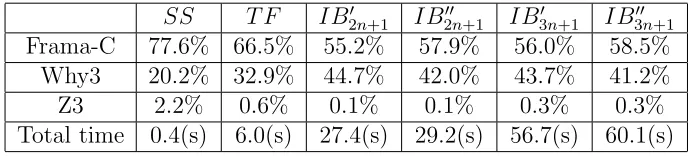
3.1 Percentage of time used by each tool in the verification

frame-work for verification of controllers of size n= 10 with inexact implementations. . . 50

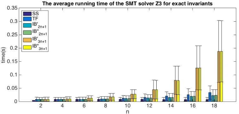
3.2 Percentage of time used by each tool in the verification

frame-work for verification of controllers of size n = 18 with exact

(16)

List of Illustrations

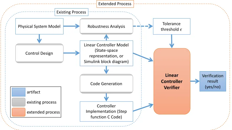
1.1 Our extended proposed process for linear controller verification 5

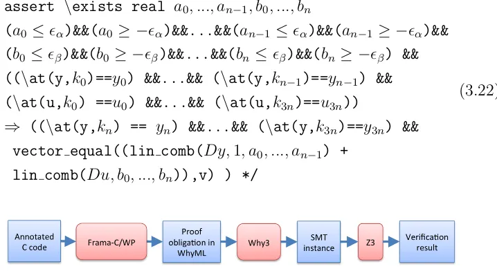
3.1 The verification toolchain of the invariant checking-based

ap-proach. . . 43

3.2 Z3 running times for LTI controller verification using five

dif-ferent types of controller invariants. . . 47

3.3 Z3 running times for verification of LTI controllers using

‘in-exact’ invariants for all five different types of controller

invari-ants. Note that in this case, verification of TF invariants does

not scale well because controllers with the size greater than

two can not be verified. . . 48

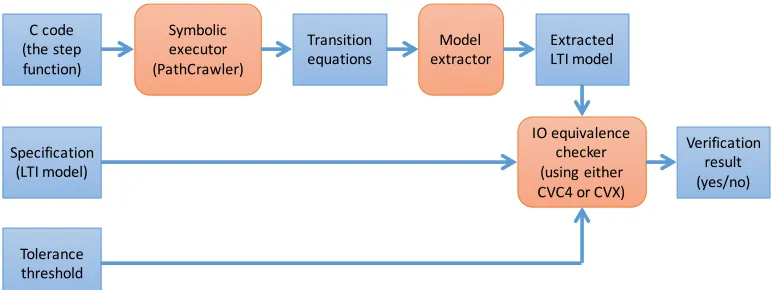
4.1 The verification toolchain for the similarity checking-based

ap-proach. . . 63

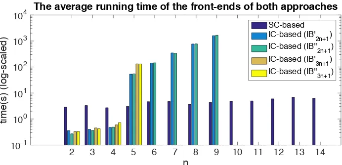
4.2 The average running time of the front-ends of both SC-based

and IC-based approaches (with the log-scaled y-axis) . . . 66

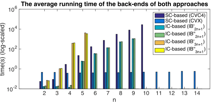
4.3 The average running time of the back-ends of both SC-based

(17)

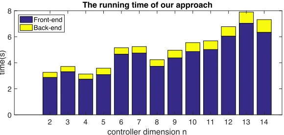
5.2 The running time of both the front-end and the back-end of

our approach . . . 84

5.3 The overhead in both the front-end and the back-end of our

approach . . . 85

6.1 The verification flow of LCV. . . 86

6.2 The simulink block diagram for checking the additivity of the

controller . . . 88

6.3 The block diagram of the PID controller. . . 92

6.4 Our quadrotor platform (Left). The quadrotor controller block

diagram (Right). . . 94

6.5 The running time of LCV for verifying controllers with

(18)

Chapter 1 Introduction

1.1 Motivation

Most safety- and life-critical embedded and cyber-physical systems have a

software-based controller at their core. The safety of these systems rely

on the correct operation of the controller. Thus, in order to have a high

assurance for such systems, it is imperative to ensure that controller software

is correctly implemented.

Nowadays, controller software is developed in a model-based fashion,

us-ing industry-standard tools such as Simulink [73] and Stateflow [77]. In this

development process, first of all, the controller model is designed and

an-alyzed. Controller design is performed using a mathematical model of the

control system that captures both the dynamics of the “plant”, the entity

to be controlled, and the controller itself. With this model, analysis is

per-formed to conclude whether the plant model adequately describes the system

(19)

control system. Once the control engineer is satisfied with the design, a

software implementation is automatically produced by code generation from

the mathematical model of the controller. Code generation tools such as

Embedded Coder [72] and Simulink Coder [74] are widely used. The

gener-ated controller implementation is either used as it is in the control system, or

sometimes transformed into another code before used for various reasons such

as numerical accuracy improvement [23, 24] and code protection [18, 15, 11].

For simplicity’s sake, we will call code generation even when code generation

is potentially followed by code transformation.

To assure the correctness of the controller implementation, it is necessary

to check that code generation is correctly done. Ideally, we would like to

have verified tools for code generation. In this case, no verification of the

controller implementation would be needed because the tools would

guaran-tee that any produced controller correctly implements its model. In practice,

however, commercial code generators are complex black-box software that

are generally not amenable to formal verification. Subtle bugs have been

found in commercially available code generators that consequently generate

incorrect code [71]. Unverified code transformers may introduce unintended

bugs in the output code.

In the absence of verified code generators, it is desirable to verify instances

of implementations against their original models. Therefore, the goal of this

work is to develop an automatic method to perform such instance verification

(20)

1.2 Problem Formulation

This work considers the problem of verifying software implementations of

controllers against controller models as mathematical specifications. We

as-sume that control design activities have been performed, achieving the

ac-ceptable degree of assurance for the control design. Thus, the mathematical

model of the controller is correct with respect to any higher-level

require-ments and can be used as the specification for a software implementation of

the controller.

Controllers are generally specified as a function that, given the current

state of the controller and a set of input sensor values, computes control

output that is sent to the system actuators and the new state of the controller.

We refer to this function as the state-space representation of the controller. In

this work, we focus on linear-time invariant (LTI) controllers, since these are

the most commonly used controllers in control systems. In LTI controllers,

the relationships between the controller input and current state values, and

the computed control output and updated state values are both linear.

In software, controllers are implemented as a subroutine (or a function

in the C language). This function is known as the step function. The step

function is invoked by the control system periodically, or upon arrival of new

sensor data (i.e., measurements).

To properly address this verification problem, the following challenges

should be considered: First of all, such verification should be performed

from the input-output perspective (i.e., input-output conformance).

Cor-rect implementations may have different state representations to each other

(21)

represen-tation, optimization used in the code generation process). In other words,

the original controller model and a correct implementation of the model may

be different from each other in state representation, while being functionally

equivalent from the input-output perspective. Thus, it is necessary to develop

the verification technique that is not sensitive to the state representation of

the controller.

Moreover, there is an inherent discrepancy between controller models and

their implementations. The controller software for embedded systems uses a

finite precision arithmetic (e.g., floating-point arithmetic) which introduces

rounding errors in the computation. The effect of these rounding errors needs

to be considered in the verification process. In addition to these rounding

errors, the implementations may be inexact in the numeric representation

of controller parameters due to the potential rounding errors in the code

generation/optimization process. Thus, it is reasonable to allow a tolerance

in the conformance verification as long as the implementation has the same

desired property to the model’s.

Finally, such verification is desired to be automatic and scalable because

verification needs to be followed by each instance of code generation. In the

next section, we describe the contributions of our proposed methods that

address this problem.

1.3 Contributions

At a high level, the goal of this work is to ensure the correctness of controller

(22)

ab-Controller Implementation (Step

function C Code) Linear Controller Model

(State-space representation, or Simulink block diagram)

Linear Controller

Verifier

Verification result (yes/no) Code Generation

Physical System Model

Control Design

Tolerance threshold !

Existing Process

Extended Process

artifact

existing process

extended process

Robustness Analysis

Figure 1.1: Our extended proposed process for linear controller verification

sence of verified code generators. Thus, as shown in Figure 1.1, we propose

an extended process building upon the existing model-based development

process. The main new entity in the extended proposed process is Linear

Controller Verifier (LCV), an automatic tool to verify a step function C code

(i.e., controller implementation) against an LTI controller model from the

input-output perspective with tolerance up to a given threshold value.1 _To develop LCV, we explore two alternative approaches in this dissertation: one

is based on invariant checking while another is based on similarity checking.

The more specific contributions that this dissertation make are as follows:

First of all, we propose an invariant checking-based verification method [58].

Given a controller model, this method derives assertions to be satisfied by

1_{We assume that a threshold value} _{is given by a control engineer as a result of}

(23)

correct step functions. These assertions exactly capture the specification of

the controller, thus the problem of verifying step function is reduced to the

problem of checking whether these assertions are invariant to the step

func-tion or not. These asserfunc-tions enable the verificafunc-tion of the input-output only

conformance, because they are stated over the input and output variables

only, and no state variables appear in the assertions. In order to do this,

we rely on a different specification of the controller that is insensitive to the

representation of control state. This representation, based on the transfer

function of the controller, relates the current control output to the series

of past control inputs. Moreover, given a tolerance threshold by a control

engineer, we provide a way to relax the invariants (i.e., assertions) of the

controller code in order to tolerate inexact controller parameters up to the

threshold. We demonstrate how the generated control code can be

auto-matically verified with respect to a given transfer function using the popular

deductive software verification framework Frama-C [22], Why3 platform [13],

and the SMT solver Z3 [26].

Secondly, we propose a similarity checking-based verification method [60].

This approach is based on extracting a model from the controller code and

establishing equivalence between the original and the extracted models. This

similarity checking-based method significantly improves the scalability of

ver-ification compared to the invariant checking-based method. The main reason

is that the similarity checking-based method symbolically executes the given

controller code only one time, thus avoiding the loop/execution unrolling that

the invariant checking-based method involves. The first step of the

(24)

code using the symbolic execution technique. The symbolic expressions

iden-tified as the result of symbolic execution are used to reconstruct the model

of the controller. Next, the reconstructed model is checked for input-output

equivalence against the given original model, using the well-known

neces-sary and sufficient condition for the equivalence of two minimal LTI models.

We account for the numerical errors of the inexact controller parameters by

allowing for a bounded discrepancy between the models in the equivalence

checking. We provide two ways to automatically check the equivalence based

on an SMT problem formulation and a convex optimization formulation

re-spectively.

Thirdly, building on the work of the similarity checking-based method,

we propose an extended verification approach that correctly accounts for

the floating-point calculation of controller implementation. In this extended

method, we newly introduce error terms into the representation of the

ex-tracted model that characterize the effects of floating-point rounding errors.

We use an optimization formulation to perform approximate equivalence

checking. We demonstrate that this extended approach suffers only

min-imal degradation in performance while offering a higher assurance of the

floating-point controller implementation.

Lastly, we develop LCV, the prototype tool in Figure 1.1 that implements

our verification approaches. The tool accepts a subset of Simulink block

diagrams (i.e., LTI) as input and performs conformance checking against the

given implementations. We demonstrate that the tool are able to detect some

known reproduced bugs of the code generator Embedded Coder [72], and an

(25)

1.4 Related Work

This section provides a brief summary of related work, and argues the

rea-son why the current techniques are insufficient in coping with the proposed

problem in this thesis. To ensure the correctness of controller

implemen-tation against the controller model, a typically used method in practice is

equivalence testing (or back-to-back testing) [70, 19, 20] which compares the

outputs of executable model and code for the common input sequence. The

limitation of this testing-based method is that it does not provide a thorough

verification.

Static analysis-based approaches [12, 34, 39] have been used to analyze

the finite-precision numerical controller code, but focuses on checking

com-mon properties such as numerical stability, the absence of buffer overflow or

arithmetic exceptions rather than verifying the code against the model.

The work of [65, 52] proposes translation validation techniques for Simulink

diagrams and the generated codes. The verification relies on the structure of

the block diagram and the code, thus being sensitive to the controller state

while our method verifies code against the model from the input-output

per-spective, not being sensitive to the controller state. Due to optimization and

transformation during a code generation process, a generated code which is

correct may have different state representation than the models. In this case,

our method can verify that the code is correct with respect to the model, but

the state-sensitive methods [65, 52] cannot.

[35, 42, 81, 80] present a control software verification approach based on

the concept of proof-carrying code. In their approach, the code annotation

(26)

code generation. The annotation asserts control theory related properties

such as stability and convergence, but not equivalence between controller

specifications and the implementations. In addition, their approach requires

the control of code generator, and may not be applicable to the off-the-shelf

black-box code generators.

There is a line of work that has focused on robust implementations of

em-bedded controllers. For instance, in [66] the authors present a model-based

simulation platform that can be used to analyze controller robustness against

different implementation issues, including sampling, quantization, and

fixed-point arithmetic. [5, 53] present methods for design of robust fixed-fixed-point

controllers that guarantee stability and minimize implementation errors,

re-spectively. In [51], the authors introduce a robustness analysis tool that

computes the maximum deviation of the plant states due to measurement

uncertainties. The use of SMT solvers for synthesis of fixed-point embedded

software has been addressed in [25, 33].

Firnally, the authors in [6] present a method for verification of Simulink

models by translating them to Why3 [13] models. Yet, the verification is

again performed only on the model level and not on the code level.

1.5 Outline of the Dissertation

The rest of this dissertation is organized as follows:

Chapter 2 provides a background of this dissertation including LTI

sys-tems with motivating examples, and an overview of software verification

(27)

Chapter 3 describes an invariant checking-based approach to verify

soft-ware implementations of LTI controllers with respect to their mathematical

specifications by transfer functions. This chapter describe a toolchain

de-veloped to perform such verification, and demonstrate the scalability of the

approach using a set of randomly generated controllers of varying sizes.

Chapter 4 presents a similarity checking-based approach to verify

con-troller implementations by extracting models from the implementations and

comparing the extracted models against the original models. This chapter

also demonstrate the scalability of the prototype tool of this approach.

Chapter 5 presents a method that extends the similarity checking-based

approach of Chapter 4. This extended method correctly accounts for the

rounding errors that would occur in the floating-point computation of the

controller implementation. We demonstrate the scalability of our proposed

approaches through evaluation with randomly generated controller

specifica-tions of realistic size.

Chapter 6 describes LCV, the prototype tool that implements our

veri-fication approaches. This chapter also evaluates the tool LCV through the

case study and the scalability analysis.

Chapter 7 concludes the dissertation and discuss future research

(28)

Chapter 2 Preliminaries

This chapter presents preliminaries on LTI controllers and their software

implementations. We also introduce two real-world examples that motivate

the problem considered in this thesis, as well as the problem statement.

2.1 Notation and Definitions

We use_Rto denote the set of reals, while matrixIndenotes then×nidentity

matrix. Theithelement of vectorxkis denoted byxk,i.1 For vectorx, we use

to denote by |x| the vector whose elements are absolute values of the initial

vector. Also, a square matrix A is called nonsingular if its determinant is

not equal to zero.

A discrete system takes a discrete-time signal uk, k ≥ 0, as input and

generates a discrete-time signal yk as output in response to the input. The

system may have a hidden internal state. In this case, the output signal yk

(29)

is influenced by not only the input signal uk but also the internal state of

the system at time k. The change of the internal state is influenced by the

input signal uk and the current internal state. A discrete system is said to

be linear if αyk+βyˆk is the output of the system in response to the input αuk+βuˆk for any scalars α and β when yk and ˆyk are the outputs of the

systems in response to the inputuk and ˆuk respectively. Moreover, a system

is said to be time-invariant if yk−k0 is the output of the system in response

to the inputuk−k0 for anyk0 whenyk is the output of the system in response

to the input uk.

Finally, for discrete-time signalxk, k≥0, the z-transform is a function of

a complex variable defined as X(z) = P∞_k₌₀xkz−k. For the signal xk in the

time domain, this z-transform produces a new presentation X(z) in the

z-domain. The z-transform is considered as the discrete analogue of the Laplace

transform [64]. Rational functions are functions that can be represented by

an algebraic fraction where both the numerator and the denominator are

polynomial functions.

2.2 Linear Feedback Controller

The goal of feedback controllers is to ensure that the closed-loop systems have

certain desired behaviors. In general, these controllers derive suitable control

inputs to the plants (i.e., systems to control) based on previously obtained

measurements of the plant outputs. In this thesis, we consider a general class

(30)

controllers in the standard state-space representation form:

zk+1 =Azk+Buk

yk=Czk+Duk.

(2.1)

where uk ∈ Rp, yk ∈ Rm and zk ∈ Rn are the input vector, the output

vector and the state vector at time k respectively. The matrices A ∈_Rn×n_,

B ∈_Rn×p_,_C_∈

Rm×n andD ∈Rm×p together with the initial controller state

z0 completely specify an LTI controller. Thus, we use Σ(A,B,C,D,z0) to denote an LTI controller, or just useΣ(A,B,C,D) when the initial controller state z0 is zero.

During the control-design phase, controller Σ(A,B,C,D,z0) is derived to guarantee the desired closed-loop performance, while taking into account

available computation and communication resources (e.g., finite-precision

arithmetic logic units). This model (i.e., controller specification) is then

usu-ally ‘mapped’ into a software implementation of a step function that: (1)

maintains the state of the controller, and updates it every time new

sen-sor measurements are available (i.e., when it’s invoked); and (2) computes

control outputs (i.e., inputs applied to the plant) from the the current

con-troller’s state and incoming sensor measurements. In most embedded control

systems, the step function is periodically invoked, or whenever new sensor

measurements arrive. In this thesis, we assume that data is exchanged with

the step function through global variables.2 _{In other words, the input, output}

and state variables are declared in the global scope, and the step function

2_{This convention is used by Embedded Coder, a code generation toolbox for}

(31)

reads both input and state variables, and updates both output and state

variables as the effect of its execution. It is worth noting however that this

assumption does not critically limit our approach because it can be easily

extended to support a different code interface for the step function.

2.3 Motivating Examples

To motivate our work, we introduce two examples, which illustrate

limita-tions of the standard verification techniques that directly utilize the

mathe-matical model from (6.1), in cases when controller software is generated by a

code generator whose optimizations potentially violate the model while still

ensuring the desired control functionality.

2.3.1 A Scalar Linear Integrator

Consider a simple controller that computes control input yk as a scaled sum

of all previous sensor data ui ∈R, i= 0, ..., k−1 – i.e.,

yk = k−1 X

i=0

αui, k >1, and, y0 = 0. (2.2)

Now, if we use the Simulink Integrator block with Forward Euler

in-tegration to implement this controller, the resulting controller model will

be Σ(1, α,1,0), – i.e., zk+1 =zk +αuk, yk =zk. On the other hand, a

real-ization ˆΣ(1,1, α,0) – i.e., zk+1 = zk+uk, yk = αzk, of the controller would

introduce a reduced computational error when finite precision arithmetics is

(32)

soft-ware implementations due to the use of different code generation tools. Still,

it is important to highlight that these two implementations would have

iden-tical input-output behavior – the only difference is whether they maintain a

scaled or unscaled sum of the previous sensor measurements.

2.3.2 Multiple-Input-Multiple-Output Controllers

Now, consider a more general Multiple-Input-Multiple-Output (MIMO)

con-troller with two inputs and two outputs which maintains five states

zk+1 =           

−0.500311 0.16751 0.028029 −0.395599 −0.652079

0.850942 0.181639 −0.29276 0.481277 0.638183

−0.458583 −0.002389 −0.154281 −0.578708 −0.769495

1.01855 0.638926 −0.668256 −0.258506 0.119959

0.100383 −0.432501 0.122727 0.82634 0.892296

          

| {z }

A

zk+

+           

1.1149 0.164423

−1.56592 0.634384 1.04856 −0.196914

1.96066 3.11571

−3.02046 −1.96087           

| {z }

B

uk (2.3)

yk =





0.283441 0.032612 −0.75658 0.085468 0.161088

−0.528786 0.050734 −0.681773 −0.432334 −1.17988 



| {z }

C

zk

(33)

The controller has to perform 25 + 10 = 35 multiplications as part of the

state z update in every invocation of the step function. On the other hand,

the following controller requires only 5 + 10 = 15 multiplications for state

update.

ˆ zk+1=

          

0.87224 0 0 0 0

0 0.366378 0 0 0

0 0 −0.540795 0 0

0 0 0 −0.332664 0

0 0 0 0 −0.204322

          

| {z }

ˆ

A

ˆ zk+

+           

0.822174 −0.438008

−0.278536 −0.824313 0.874484 0.858857

−0.117628 −0.506362

−0.955459 −0.622498           

| {z }

ˆ

B

uk, (2.5)

yk=





−0.793176 0.154365 −0.377883 −0.360608 −0.142123

0.503767 −0.573538 0.170245 −0.583312 −0.56603





| {z }

ˆ

C

ˆ zk

(2.6)

The above controllers Σ and ˆΣ are similar, which means that the same

input sequences yk delivered to both controllers, would result in identical

(34)

dif-fer. Consequently, the ‘diagonalized’ controller ˆΣ results in the same control

performance and thus provides the same control functionality as Σ, while

violating the state evolution model of the initial controller Σ. The

moti-vation for the use of the diagonalized controller comes from a significantly

reduced computational cost that allow for the utilization of resource

con-strained embedded platforms. In general, any controller (6.1), would require

n2 ₊_np ₌ _n₍_n ₊_p_{) multiplications to update its state. This can be}

sig-nificantly reduced when matrix A in (6.1) is diagonal – in this case only

n+np =n(p+ 1) multiplications are needed.

2.4 Software Verification Techniques

This section briefly overviews the software verification techniques such as

deductive verification, symbolic execution and model extraction.

2.4.1 Deductive Verification

Deductive verification [36] is a deductive approach to verify a program, which

normally consists of two steps: (1) turning the correctness of a program into

a mathematical statement (also known as verification condition), and then

(2) proving the statement. The correctness of a program is defined by a

specification of the program. A specification can be given using the concept

of Hoare triple [43]. A Hoare triple is the form {P}s{Q} where P is a

pre-condition, s is a program statement, and Q is a postcondition. A program

statement s is said to be correct with respect to some given precondition P

(35)

triple {P}s{Q} is valid if the execution of s starting from any state that satisfies P finishes in a state that satisfies Q. Note that if s is not termi-nating, it is correct for any P and Q. In this regard, the validity of a Hoare

triple asserts the partial correctness of a program. An additional

require-ment for s to be terminating defines total correctness. One can establish

the validity of a Hoare triple using the Hoare rules with providing proper

intermediate assertions. However, this typically requires much manual effort

in practice. Thus, most modern verification condition generators use the

weakest precondition calculation which computes the weakest precondition

wp(s, Q) for some given program statements and postconditionQsuch that

{wp(s, Q)}s{Q}. Consequently, the validity of the Hoare triple {P}s{Q}

is equivalent to P =⇒ wp(s, Q). Generated verification conditions can

be discharged by the support of tools such as SMT solvers (e.g., Z3 [26],

CVC4 [8]) and interactive theorem provers (e.g., Coq [7], PVS [57]), possibly

being coordinated by a multi-prover deductive verification framework [37].

Finally, Frama-C [22] and ACSL [10] have been widely used for software

verification. For example, for verification of a subset of the standard C

library [16], safety-critical software in the railway domain [41], and the Xen

kernel [63]). In addition, [28, 48] present methods for dynamic analysis in

Frama-C, and in [42] the authors present the use of Frama-C for verification

of control software.

2.4.2 Symbolic Execution

Symbolic execution [47] [17] is a program analysis technique which executes a

(36)

Symbolic execution contrasts with concrete execution. Concrete execution

for program analysis can be said to be program testing, which process is as

follows: concrete values are given as an input to a program under test. The

program is executed for the concrete inputs, and the observable behavior

(e.g., output) of the execution is inspected to see if it is expected or not.

In this process, a concrete execution yields a single execution path. In most

cases, concrete executions only cover a small subset of the whole input space,

and thus may miss the program executions which actually lead to errors.

On the other hand, symbolic execution allows a program to take as

in-put symbolic values instead of concrete values. A symbolic value (e.g., α,

β) denotes an arbitrary concrete value. For a given symbolic input, a

sym-bolic execution engine explores the control flow paths of the program while

maintaining (1) a symbolic program state which maps variables to symbolic

expressions, and (2) a path condition which is a constraint on the symbolic

input values and characterizes the path currently being explored. In other

words, a path condition is the conjunction of the conditions of the branches

taken along the path. During a symbolic execution, branch statements

up-date the path condition, while assignment statements upup-date the symbolic

program state.

Symbolic execution can be used in program analysis in many different

ways. First of all, symbolic execution can be used to generate test cases that

covers certain execution paths. Suppose that there is an execution path with

path condition C. The feasibility of the path is reduced to the satisfiability of the path condition C. Constraint solvers (e.g., Z3 [26] and CVC4 [8]) are

(37)

as a concrete input (i.e., test case) that covers the path. Moreover, symbolic

execution can be used to verify assertions in programs. Suppose that the path

with the path condition C reaches an assertion statement which asserts the

predicate P. If (C =⇒ P) is valid, it is guaranteed that all concrete input values that lead to the path (i.e., satisfies C) are not violating the assertion

P. Checking the validity of the formula can also be done automatically

by constraint solvers. If the formula is not valid, the solvers also provide

a concrete assignment (i.e., concrete input value) that causes the assertion

violation.

2.4.3 Model Extraction

The model extraction technique has been used in software verification [78,

21, 45, 46, 54, 79, 62, 67]. There is a line of work that has focused on

using the model extraction technique for software model checking [78, 21,

45, 46, 54]. From a given source program, these model extraction tools

automatically extract a verification model in the input language of several

existing model checkers such as SPIN [44], SMV [55], SAL [27] and Zing [4].

Bandera [21] takes Java programs, and extracts models from the programs

in a certain intermediate representation which are further translated into the

input languages of existing model checkers such as SPIN, SMV and SAL.

Modex [45, 46] extract the control-flow skeleton of a given C program in

the Promela language [44] to verify the message passing operations of the

program using the SPIN model checker. The work [54] focuses on extracting

verification models from C programs of Windows kernel drivers to facilitate

(38)

There is also much work on extracting high-level state machine models

from source programs [49, 69, 79, 67]. These approaches reconstruct a state

machine model from a given program for the use of program testing and

code review (i.e., visualizing the state machine model for a programmer to

understand the high-level perspective of the behavior of the legacy program).

For model extraction, the symbolic execution technique is used in [49, 79, 67]

while the work [69] analyze the structure of the abstract syntax tree of the

program.

Finally, the work [62] applies the symbolic execution technique to

im-plemented source code to extract mathematical functional models. The

ap-proach only considers a restricted set of programs that can be represented as

pure mathematical functions (i.e., without having states), thus being unable

to account for persistent static variables such as global variables which are

(39)

Chapter 3 Invariant Checking-based

Verification Approach

This chapter describe an invariant checking-based verification method [58].

Given a controller model, this method derives assertions to be satisfied by

correct step functions. These assertions exactly capture the specification of

the controller, thus the step function verification problem is reduced to the

problem of checking whether these assertions are invariant to the step

func-tion or not. In order to derive invariants that assert the input-output only

conformance of code against model, we rely on a different specification of the

controller that is insensitive to the representation of control state. This

repre-sentation, based on thetransfer function of the controller, relates the current

control output to the series of past control inputs. The number of past inputs

needed to capture the transfer function is known as the degree of the

con-troller. It is well known that every state-space representation of a controller

(40)

simi-lar) state-space representations will have the same transfer function [64]. In

this chapter, we demonstrate how the generated control code can be

auto-matically verified with respect to a given transfer function using the popular

software verification framework Frama-C [22], Why3 platform [13], and the

SMT solver Z3 [26].

Verification is currently performed in the domain of real numbers,

disre-garding numerical errors due to floating point calculations in the software.

We are planning to address the floating point domain in our future work.

As the first step towards the full treatment of the problem, we consider

im-precise implementations of the controller and allow coefficients of its transfer

function to deviate from the specification, up to a fixed bound. We show

that, while these bounded-error specifications can be handled using the same

tool chain as exact specifications, they yield SMT problems with a

differ-ent structure, which adversely affect scalability of the solution. We then

propose an alternative, equivalent specification for the controller, which we

call an instantiation-based specification. We show that by slightly increasing

the size of the specification, we can dramatically improve the scalability of

verification.

This chapter is organized as follows: Section 3.1 introduces invariants

for linear controllers and methods for code annotation, for both exact and

inexact controller implementations. In Sec. 3.2, we define instantiation-based

invariants for linear controllers. Finally, in Sec. 3.3, we present the developed

(41)

3.1 Defining Invariants for Linear Controllers

In this section, we introduce invariants for linear controllers that can be used

to verify both state and input-output conformance of the obtained code or

onlyinput-output conformanceof the code. By the input-output conformance

we refer to the requirement that in response to provided inputs the code

provides outputs equal to the outputs provided by the model in (6.1) for the

same input signals. Additionally, by state and input-output conformance we

refer to the requirement that in response to provided inputs the code fully

conforms to the initial model in (6.1) – i.e., not only in output but also in

the internal state of the controller.

Accordingly, for verification of state and input-output (IO) conformance,

invariants can be directly obtained from the model in (6.1). On the other

hand, as illustrated in the previous section, there is a need to provide a

method to capture input-output (IO) only invariants for linear controllers.

These invariants cannot utilize any assertions on the controller’s state,

be-cause controller implementations may be equivalent from the input-output

perspective and yet rely on different state representations.

3.1.1 Input-Output Invariants

We consider a controller defined as Σ = (A,B,C,D). The controller’s trans-fer function G(z), defined as G(z) = _UY(₍_zz)₎ where U(z) and Y(z) denote the

z-transforms of the signals uk and yk respectively, is a convenient way to

(42)

For the controller Σ we have that

G(z) = C(zIn−A)−1B+D. (3.1)

In general, G(z) is a m×p matrix with each element Gi,j(z) being a

ra-tional function of the complex variable z. To simplify the notation, unless

otherwise noted, we will assume that the considered controller is a

Single-Input-Single-Output (SISO) controller, meaning that the transfer function

G(z) is a (single, not a matrix) rational function of z. The introduced in-variants can be easily extended to Multiple-Input-Multiple-Output (MIMO)

controllers.

From (3.1), in the general case G(z) takes the form

G(z) = β0 +β1z

−1₊_{· · ·}₊_β

nz−n

1 +α1z−1+· · ·+αnz−n

, (3.2)

where n is the size of the initial controller model, and we will also refer to n

as the degree of the transfer function. In addition, β0, ..., βn, α1, ..., αn ∈ R

and can be obtained as in (3.1), from the parameters of the initial controller

specification (6.1). Therefore, the transfer function is fully described by

the vectors α, β ∈ _Rn+1 _{that are defined as} _α _{= [1}_{, α}

1, ..., αn] and β =

[β0, β1, ..., βn].

From the properties of the z-transforms such as linearity and time-invariance,

the above equation implies that the controller’s input and output signals

sat-isfy the following difference equation [64]:

yk =

n

X

βiuk−i− n

X

(43)

with yk = 0, k < 0, because z0 = 0 and uk = 0, for k < 0. The coefficients

α and β of this equation come from (3.2). Thus, for any controller Σ it

is possible to obtain a linear invariant of the form in (3.3) that specifies

the relationship between controller inputs and outputs. In addition, since

transfer functions are invariant to similarity transformations [64], besides the

controller Σ, the linear invariant in (3.3) is also satisfied by any controller

ˆ

Σ obtained from the initial controller model Σ using a similarity transform

with a nonsingular matrix T.

3.1.2 Annotating Controller Invariants in C Code

The linear conditions in (6.1) and (3.3) respectively capture the expected

state and input-output, and input-output only invariants for LTI controllers.

The next challenge is to find a suitable method to express them as C code

annotations, compatible with existing verification tools. To achieve this goal,

we exploit ANSI/ISO C Specification Language (ACSL) [10] that enables

users to specify desired properties of C code within the program’s comments.

ACSL is integrated in the Frama-C platform [22] that supports tools for

reasoning about correctness of C code and incorporated ACSL annotations.

To illustrate the use of ACSL to capture C code invariants, as a running

example we use the following Σ(A,B,C,0) controller

A =





0.8147 1.1534 2.6413 3.6411 

,B =



 3.1019 2.1432 

,C=

h

1.7121 0.1351 i

(3.4)

G(z) = 5.60030931z

−1₋₁₄_._233777166248_z−2

(44)

For completeness, we first introduce annotations that capture both IO and

state conformance, before introducing IO only annotations.

3.1.3 Annotating Input-Output and State Invariants

To capture the input-output and state requirements for a C function, we

ex-ploit the ACSL’s notion of the function contract, which is effectively a Hoare

triple [43, 30] for the entire function. ACSL utilizes the keywords requires

andensuresto specify the preconditions and postconditions; the verification

goal is to prove that postconditions are satisfied upon return if preconditions

were satisfied when the function call occurred. The precondition for the

con-troller’s step function is that all pointers to memory locations are valid –

for example, valid pointers to state vectors and matrix coefficients if the

co-efficients are not directly instantiated. This requirement is supported by the

predicate valid that is part of ACSL.

On the other hand, the specified postconditions follow directly from the

linear invariants (i.e., the model) of the controller step function in (6.1).

To capture them and properly annotate the code, we exploit the built-in

ACSL predicate old that denotes the values of a variable before the code

is executed. For instance, for the considered controller defined in (3.4), the

controller code with the annotations is presented in Listing 1.

3.1.4 Annotating Input-Output Only Invariants

Unlike the state and IO invariants, the IO only controller invariants from (3.3)

(45)

double x[2], u, y;

/*@ requires \valid(x+(0..1));

@ ensures x[0] == 0.8147*\old(x[0]) +

@ 1.1534*\old(x[1]) + 3.10191*\old(u); @ ensures x[1] == 2.6413*\old(x[0]) +

@ 3.6411*\old(x[1]) + 2.1432*\old(u); @ ensures y == 1.7121*\old(x[0]) +

@ 0.1351*\old(x[1]) + 0*\old(u); */

void step() {

double t1, t2;

y = 1.7121*x[0] + 0.1351*x[1];

t1 = 0.8147*x[0] + 1.1534*x[1] + 3.1019*u; t2 = 2.6413*x[0] + 3.6411*x[1] + 2.1432*u; x[0] = t1;

x[1] = t2; }

(46)

relates the lastn+ 1 executions of thestepfunction. Therefore, to verify IO conformance of the controller code we have to perform execution unrolling of

the step function a certain number of times. To achieve this, we construct

the functionverif driverthat invokes thestepfunction exactlyn+1 times.

It is important to note here that the number of times the code needs to be

unrolled is equal to the size of the initial controller model (i.e., the degree of

transfer function) increased by 1. Finally, by using a separate label for every

step function execution, we can then exploit the built-in ACSL keyword at

to capture the values of input and output variables at each point of time

(i.e., execution of the ‘unrolled’ function).

ACSL supports assertions at the end of any C code block using theassert

keyword, where assert p specifies that p has to hold in the current state

(i.e., at the place where the assertion occurs) [10]. Thus, the invariant (3.3)

can be specified as1

/*@ assert \at(y,kn) + α1*\at(y,kn−1)+... @ αn*\at(y,k0) == β0*\at(u,kn) +...

@ βn*\at(u,k0) */

(3.6)

For instance, for controller Σ specified as in (3.4), Listing 2 presents the

verif driver function with the corresponding annotations.

1_{If the} _step _{function could change the input variables, we would have to introduce}

separate labels for inputs and outputs (instead of a single set ofk0toknpoints). However,

(47)

extern double input();

void verif_driver() { u = input(); step(); k0:;

u = input(); step(); k1:;

/*@assert \at(y,k2) - 4.4558*\at(y, k1) @ - 0.08007125*\at(y, k0)

@ == 5.60030931*\at(u, k1) @ - 14.233777166248*\at(u, k0); @ */

}

(48)

3.1.5 Inexact Controller Implementations

Let us revisit the example controller with the initial model defined in (3.4).

We obtained a computationally more efficient controller ˆΣ( ˆA,Bˆ,Cˆ,0) via a similarity transformation from the initial controller Σ; this was done in

Mat-lab using the function canon for the modal type of decomposition, resulting

in controller ˆΣ:

ˆ

A=





−0.0179 0

0 4.474



,Bˆ = 



−1.051

−1.055 

,Cˆ = h

−3.037 −2.283 i

(3.7)

ˆ

G(z) = 5.600452z

−1 ₋₁₄_._2373891245_z−2

1−4.4561z−1₋₀_._0800846_z−2 (3.8)

There exists a discrepancy between transfer functions G(z) in (3.5) and ˆ

G(z) in (3.8), which implies that that the previously introduced input-output invariant from (3.3) will not be satisfied by the control code implementing

controller ˆΣ. Although a similarity transform results in a new controller

with the same transfer function, due to finite-precision computation of the

code generator performing controller optimization (in this case Matlab), it is

possible (and expected) that the transfer function of the produced controller

slightly differs from the transfer function of the initial controller.

Consequently, there is a need to extend our input-output invariants for

the case with imprecise specification of the transfer functions. Specifically,

we extend (3.2) by assuming that the transfer function could take the form

as

G(z) = βˆ0 + ˆβ1z

−1₊_{· · ·}_{+ ˆ}_β

nz−n

1 + ˆα1z−1+· · ·+ ˆαnz−n

(49)

such that for i= 0,1, ..., n

βi−β ≤βiˆ ≤βi+β, αi−α ≤αiˆ ≤αi+α. (3.10)

Here, β and α denote the bounds on the errors of the transfer function

coefficients. We assume that these are inputs to our verification procedure;

suitable error bounds that guarantee the desired control performance can be

extracted using methods from robust control theory [31].

Yet, these inaccuracies also affect the input-output controller invariants

that now need to be (re)stated. We start by noting that from (3.9) it holds

that

∃∆βi,∆αi ∈R, i= 0, ..., n, |∆βi| ≤β ∧ |∆αi| ≤α∧

yk= n

X

i=0

(βi+ ∆βi)uk−i− n

X

i=1

(αi+ ∆αi)yk−i.

(3.11)

However, the above condition is not linear, but rather bilinear, as it

con-tains products ∆βiuk−i and ∆αiyk−i. Hence, we introduce additional

vari-ables ˜uk−i = ∆βiuk−i and ˜yk−i = ∆αiyk−i and restate (3.11) as follows

∃u˜k−i,y˜k−i ∈R, i= 0,1, ..., n,

|u˜k−i| ≤β|uk−i| ∧ |y˜k−i| ≤α|yk−i| ∧

yk = n

X

i=0

(βiuk−i+ ˜uk−i)− n

X

i=1

(αiyk−i+ ˜yk−i)

(3.12)

Sinceα≥0, the condition |y˜i| ≤α|ui| is equivalent to

(50)

A similar term can be obtained for |u˜i| ≤β|ui|. Thus, we introduce a

pred-icate error bound(a,b,c) as

#define error bound(a,b,c) (((b)>=0 && -(b)*(c) <= (a) <= (b)*(c))

|| ((b)<0 && (b)*(c) <= (a) <= -(b)*(c)))

With the above notation, and using the ACSL keyword exists for the

existential quantifier, the input-output invariant (3.12) can be annotated in

code as follows:

/*@ assert \exists real y˜0, ...,y˜n−1,u˜0, ...,u˜n

@ error bound(˜y0,\at(y,k0),α) && ... &&

@ error bound(˜yn−1,\at(y,kn−1),α) &&

@ error bound(˜u0,\at(u,k0),β) && ... &&

@ error bound(˜un,\at(u,kn),β) &&

@ (\at(y,kn)+α1*\at(y,kn−1)+˜yn−1+...+αn*\at(y,k0)+˜y0 @ == β0*\at(u,kn)+˜un+...+βn*\at(u,k0)+˜u0) */

(3.13)

For example, for the controller Σ specified (3.4), Listing 3 illustrates the

verif driver function with the input-output invariant annotations that

al-low for transfer function inaccuracies.

It is important to highlight that the IO invariant in (3.12) and the

corre-sponding code annotation in (3.13) exploit a mixture of both universal and

existential quantifiers. Existential quantifiers are used to specify tolerance

(51)

of formulas with both universal and existential quantifiers usually presents

a challenge for SMT solvers (e.g., Z3), which, as we will illustrate in the

evaluation section later (Section 3.3.1), significantly limits scalability of the

approach and degrees of controllers that can be verified using the invariant.

We address this problem in the next section as we provide another approach

to derive input-output invariants for LTI controllers.

3.2 Instantiation-based Input-Output

Invari-ants for LTI Controllers

In this section, we present an alternative method to specify linear invariants

that are equivalent to the IO invariant introduced in (3.3), (3.12) and (3.13).

As we will show, the method is better suited to capture robust invariants

that allow for slightly inexact controller implementations, as in cases when

there exists a small discrepancy between the transfer function of the initial

controller and the one implemented by the provided code.

Initially, we consider the exact input-output invariants from (3.3), and we

start by logically ‘unrolling’ the condition (3.3)N times – by summarizingN

executions of the controller from (3.3) using the matrices introduced below.

Definition. Consider controller Σ. For the controller’s inputs and outputs

(52)

extern double input();

void verif_driver() { u = input(); step(); k0:;

/*@assert \exists real yt0, yt1, ut0, ut1; @ error_bound(yt0, \at(y, k0), 0.01) && @ error_bound(yt1, \at(y, k1), 0.01) && @ error_bound(ut0, \at(u, k0), 0.01) && @ error_bound(ut1, \at(u, k1), 0.01) && @ \at(y,k2)

@ - 4.4558*\at(y, k1) + yt1 @ - 0.08007125*\at(y, k0) + yt0 @ == 5.60030931*\at(u, k1) + ut1 @ - 14.233777166248*\at(u, k0) + ut0; @ */

}

Listing 3: Annotated code for verification of the IO conformance within the

tolerance limit for the example controller from (3.4); Note that ˜y and ˜u

(53)

h

Dy_N Du

N

i where

Dy_N =        

yn yn−1 ... y1 y0

yn+1 yn ... y2 y1 ..

. ... . .. ... ...

yn+N−1 yn+N−1 ... yN yN−1         (3.14)

Du_N =        

un un−1 ... u1 u0

un+1 un ... u2 u1 ..

. ... . .. ... ...

un+N−1 un+N−2 ... uN uN−1         (3.15)

Consequently, from (3.3) and the above definition it follows that

DN ·θ =0, (3.16)

where θ = h1 α1 ... αn β0 β1 ... βn

iT

= hαT βT

iT

captures all of

the parameters of the controller’s transfer function.

The following proposition shows that under certain conditions, linear

equalities from (3.16) are equivalent to the invariant in (3.3) obtained from

the controller’s transfer function.

Proposition 1. Consider LTI controller Σ of size n. Then the rank of any

matrix DN cannot be larger than 2n+ 1. Furthermore, when the rank of DN

is 2n+ 1, then linear conditions from (3.16) are satisfied if and only if the condition (3.3) is satisfied for all k.

(54)

matrix has 2n+ 2 columns. Note that the matrix cannot have rank 2n+ 2 as

that would imply that the columns of DN are linearly independent and thus

their linear combination Dy_N ·θ could be equal to the zero vector only if all elements of θ are zero (i.e., θ =0). This is clearly not possible since 1 is the first element of θ.

Now suppose that rank(DN) = 2n+ 1. As we argued before, from (3.3)

and Definition 3.2 we have that (3.16) is satisfied. Thus, let’s consider the

other direction.

We start by assuming that (3.16) holds for a vectorθ obtained from some

vectors α and β. Since Σ is an LTI controller of size n then, as presented in Section 3.1, there exist vectors ˆα,βˆ, and ˆθ = hαˆT _β_ˆTi

T

for which (3.3) is

satisfied for each k. Therefore, since DN captures inputs and outputs of the

system (from its definition), we have that

DN ·θˆ=0=DN ·θ ⇒DN ·(θ−θˆ) = 0. (3.17)

Note that since the first element ofθ−θˆis zero,DN·(θ−θˆ) presents linear

combination of all columns of DN except the first one. Thus, from (3.17), if

θ 6= ˆθ it follows that the remaining 2n+ 1 columns of DN (i.e., without the

first column) are linearly dependent. On the other hand, the first column of

DN presents a linear combination of other columns with coefficients from ˆθ.

Thus, since the rank of DN is 2n+ 1, we have that the remaining 2n + 1

columns are linearly independent, which contradicts are previous conclusion.

(55)

The specific structure of matrix DN (the matrices with structure such

as Dy_N and Du_N are called Toeplitz matrices) makes it suitable to obtain the

rank of DN equal to 2n + 1 with exactly N = 2n + 1 rows. To generate

matrix D2n+1 with rank 2n+ 1, we start by assigning yk = 0 anduk = 0 for

all k = 0, ..., n−1, and then un = 1. After this, the only assignments are

done on uk, k > n, as the values for yk, k > n are derived from the initial

controller model (i.e., specification). Specifically, after assigning un = 1, we

set the next n−1 inputs to zero. Since n is the size of the initial controller

(which is minimal by our assumption), the corresponding firstnrows of both

Dy andDu will be linearly independent. Finally, the lastn+ 1 inputsuk, k=

2n, ...,3n, are assigned in a way that ensures that each newly introduced row is linearly independent of the previous ones – this is easy to achieve due to

the fact that inputs uk, k=n+ 1, ...,2n−1 were all zero.

The above proposition allows us to specify a set of 2n+1 linear invariants, which if satisfied would verify input-output conformance of the considered

controller code – i.e., the invariant in (3.3). At first glance, the benefits of

using the invariant with 2n+ 1 linear conditions might be unclear, when an

invariant with a single linear condition can be used. However, as we discussed

at the end of the previous section, the invariant in (3.3) and its corresponding

ACSL annotation (3.6) require that for all values ofuat pointsk0... knandy

atk0 ... kn−1, the value ofyatkn is equal to the specified linear combination

of uk’s and yk’s. On the other hand, the invariant (3.16) does not use the

universal quantifier; rather, it specifies that if values of uk at 3n+ 1 points

are equal to the corresponding values from Du₂_n₊₁ and the values of yk at

Automatic Verification Of Linear Controller Software

University of Pennsylvania

ScholarlyCommons

Automatic Verification Of Linear Controller

Software

Junkil Park

Automatic Verification Of Linear Controller Software

Acknowledgements

Contents

List of Tables

List of Illustrations

Chapter 1

Introduction

1.1

Motivation

1.2

Problem Formulation

1.3

Contributions

1.4

Related Work

1.5

Outline of the Dissertation

Chapter 2

Preliminaries

2.1

Notation and Definitions

2.2

Linear Feedback Controller

2.3

Motivating Examples

2.3.1

A Scalar Linear Integrator

2.3.2

Multiple-Input-Multiple-Output Controllers

2.4

Software Verification Techniques

2.4.1

Deductive Verification

2.4.2

Symbolic Execution

2.4.3

Model Extraction

Chapter 3

Invariant Checking-based

Verification Approach

3.1

Defining Invariants for Linear Controllers

3.1.1

Input-Output Invariants

3.1.2

Annotating Controller Invariants in C Code

3.1.3

Annotating Input-Output and State Invariants

3.1.4

Annotating Input-Output Only Invariants

3.1.5

Inexact Controller Implementations

3.2

Instantiation-based Input-Output

Invari-ants for LTI Controllers