Evaluation of water uptake functions under salinity and
water stress conditions in turf grass
Soodabeh Seifi
1, Mohammad Bakhshi
2*
and Amin Alizadeh
31
Irrigation and Drainage Engineering Department, Agriculture Faculty, Ferdowsi University, Mashhad, Iran.
2
Environmental Sciences Faculty, Technische Universität Dresden, Dresden, Germany.
3
Agriculture Faculty, Ferdowsi University, Mashhad, Iran.
Accepted 10 July, 2019
ABSTRACT
Iran is located in arid and semi-arid region in the world which is faced with drought and salinity problems in the field of irrigation. In this situation, the water productivity is lower than the global average amount. One of useful management tool is mathematical models which simulated the relationship between farmland variables (e.g. accessible soil moisture) and amount of plant transpiration. There are different mathematical models to express the reaction of plants in simultaneous drought and salinity stresses conditions and their portion in water uptake reduction. In this study, six macroscopic water uptake reduction functions are evaluated on Lolium perenne by greenhouse data, Van Genuchten (1987) (additive and multiplicative), Dirksen and Augustijn (1988), Van Dam et al. (1997), Homaee (1999) and Skaggs et al. (2006). The experiment was done as a factorial version in a random plan with four levels of salinity (0.5, 5.5, 7.5 and 10 ds/m) and three levels of drought (100, 75 and 50 percent of field capacity) and in three repetitions. The results revealed that the reaction of Lolium perenne in low salinity level to coincident salinity and drought stresses is an additive agreement, while at the salinity level above 5.5 ds/m, the multiplicative models have a better agreement. Among all multiplicative models, the models of Skaggs et al., Homaee and Van Genuchten have a finer agreement.
Keywords: Drought stress, Lolium perenne, salinity stress, water uptake model.
*Corresponding author. E-mail: [email protected]. Tel: +989154792575.
INTRODUCTION
Drought and soil salinity are significant production limitation in arid and semi-arid regions (Homaee, 1999). Root water uptake is a dynamic term which influenced by soil, plant, and climate and related to some factors such as soil hydraulic conductivity, root depth, density distribution, soil-water pressure head, and osmosis head, evaporation requirement, water table, plant resistance, and growth stage. Therefore, it is complicated to express an exact physical explanation in water uptake (Skaggs et al., 2006). If the simulated water uptake models can predict the water flow to roots exactly, then the irrigation times can be calculated to maximize plant growth by considering the physical and chemical properties of water and soil and plant characters (Green et al., 2006).
Cardon and Letey (1992) indicated that almost, all
mathematical models of water and salts movements in soil have released via calculated numerical equation of Darcy-Richards in terms of water uptake for vertical flow. Since the plant water uptake occurred in a non-saturated soil, hence it should be considered in the Richards equation is converted to a new style (Equation 1) when the plant water uptake took into account:
K
h
S
z
h
h
K
z
t
(1)
Where θ is the volumetric soil moisture, t is the time (s), z is the depth (m), K is the drainage coefficient of unsaturated soil (ms-1), h is the matric potential (m) and S
ISSN: 2315-9766
is the amount of water that is uptake by plant roots in a unit of soil volume and time (m3m-3s-1). There are two methods to mathematical simulate of the amount of S.
The first method is based on a single root model that has been used in the microscopic scale. The second method is the root system model which considers whole roots and has been used in the macroscopic scale. The microscopic models are formed in corresponding the rate of water uptake with soil drainage coefficient and the difference between root surface matric potential and surrounded soil. Each separated soil is assumed a uniformed infinite length cylinder that has the same properties in each section, in the mentioned definition. Gardner (1960) is the pioneer investigator of general equation of microscopic water uptake models and after him the extensive studied were occurred by Whisler et al. (1968), Nimah and Hanks (1973), Feddes et al. (1974), Childs and Hanks (1975), Hansen et al. (1974a, 1974b), Van Bavel and Ahmed (1976), Herkelrath et al. (1977), Rowse et al. (1978) and Bresler et al. (1982). The main drawback of microscopic models is related to their unworkability because their quantities are inaccessible. Moreover, some basic assumptions of these models are no logical such as the uniformity of absorption location on the root level and the permanent water flow (Mathur and Rao, 1999). The first assumptions of macroscopic models were funded by Molz and Remson (1970, 1971) which remark the relationship between root water uptake and actual plant transpiration. Feddes et al. (1976, 1974) defined the new term in reducing water uptake which made the macroscopic models more generalized. His first general macroscopic model is illustrated in below:
r p
Z T h S
h
S
,
max
,
(2)Where the α(h,π) is the responsible dimensionless function of stress, Tp is the potential transpiration rate (m)
and Zr is the depth of the root zone (m) .
The famous macroscopic models are expressed by Equation 3. When the transpiration is more than water uptake, the water stress occurs. If there is no water limitation in the soil, the amount of water uptake is equal to potential of transpiration and the general equation is as Equation 3.
r p
Z T S
S max (3)
If the soil cannot prepare enough water for the plant which is equal to the maximum amount of transpiration, then the transpiration rate is reduced by the amount of α that is called transpiration reduction function.
h
S
S
max
Tp Tmax
h (4)Feddes et al. (1976) was assumed that the amount of water uptake is maximal when the absolute value of soil water pressure head (|h|) is between h2 and h3 (Figure 1).
According to this figure, by increasing the absolute value of “h” from |h3| to |h4| which is the soil matric potential in
the wilted point moisture, the water uptakes is gently declined linearly and reach to zero at the end. The water uptake in |h1| is zero because of soil saturated and
oxygen deficit. Moreover, the |h3| is a function of capillary
transpiration demand, when the demand is increased then the amount of |h3| is decreased (Denmead and
Shaw, 1962).
The other famous water uptake reduction function due to drought stress is the sigmoid reduction function of Van Genuchten.
ph
h
h
50
1
1
(5)Where the h50 is the matric potential when the amount of
water uptake is decreased by 50 percent and the p is the experimental parameter equal to 3 which is related to the plant, soil and continental condition.
Dirksen et al. (1993) have been moderated the Van Genuchten equation to the amount of reduction threshold of matric potential (h*).
ph
h
h
h
50 *
*
1
1
(6)If in place of α(h), the reduction coefficient is set by the
function of soil soluble osmosis potential, then the water uptake equation of salinity soils is converted to Equation 7.
S
maxS
(7)Where the α(π) is the water uptake reduction function due
to salinity stress. The Maas and Hoffman (1977) model and sigmoid model of Van Genuchten and Hoffman (1984) are two well-known simulated models of water uptake in salinity soils.
Figure 1. The schematic figure of reduction function of water uptake by root (Feddes et al., 1978).
and salinity stresses have been studied separately, the reduction amount of water uptake by the plant when both stresses occur was unanswered. Many theories and models are available regarding to the reaction of plants in the simultaneous salinity and drought stresses conditions and their portions at the water uptake reduction, which are divided into additive and multiplicative models. In additive models, the water uptake is assumed as a result of weight aggregate the soil-water pressure and osmosis pressure. On the other side, the reduction coefficient of salinity and water stress are calculated separately and multiplicities together finally, in the multiplicative models.
Obviously, the grass plays a significant role in the green grassland; consequently, the aim of this project is identified as the reduction of Lolium perenne to the salinity and water stress conditions, furthermore, evaluation of the mentioned models.
MATERIALS AND METHODS
Experimental plan and location
This study occurred at research greenhouse of Agriculture faculty of Ferdowsi University from January until June 2013. In this research, a complete randomized factorial design with three repetitions and in greenhouse condition on Lolium perenne was done to evaluate the water uptake simulation models in the variable condition of osmosis and matric potential. The experimental treatments contained four levels of salinity (0.5, 5.5, 7.5 and 10 ds/m) and three levels of drought (100, 75, 50 percent of field capacity). The whole pots filled by loamy gray texture and equal weight.
Methods
In this investigation, each pot was a polyethylene pipe with 11cm as diameter and 70cm as height. After spent the growing period of
Lolium perenne (3 months) and covered the whole surface of each
pot (eliminate the transpiration from the surface), the salinity and water stress executed coincidentally. The drought stress was applied in terms of field capacity percentage. Salinity level was achieved by dissolving the different amount of salt (NaCl) in one liter of water and try and error method of EC-meter equipment. Each pot was weighted daily (at 10 A.M.) with an accurate scale (accuracy equal to 0.001 kg) and once in two days, the required water was applied, according to each experimental treatment when this process was exerted for one month.
To measure the matric potential, the soil-water retention curve by pressure plate equipment and RETC (RETention Curve) software was achieved (Figure 2), firstly, and then the absolute value of matric potential was calculated by substituting the amounts of measured daily moisture
The volume of daily transpiration obtained by measuring the difference of each pot weight in respect two days and reduction coefficient of water uptake which was gotten by dividing the daily transpiration and potential transpiration (when the plant growth without any stress).
Figure 2. The soil-water retention curve.
Applied models
In this research, three reduction function in drought stress condition and six functions in coincident stresses (drought and salinity) condition with greenhouse data on Lolium perenne were evaluated. The applied reduction functions of drought stress were innovated by Feddes et al. (1976) as M7, Van Genuchten and Hoffman (1984) as
M8 and Dirksen et al. (1993) as M9, moreover the functions of
drought and salinity simultaneously were achieved by Van Genuchten (1987) (additive and multiplicative), Dirksen and Augustijn (1988), Van Dam at al. (1997), Homaee (1999) and Skaggs et al. (2006).
- The additive model of Van Genuchten (1987) as M1:
z
t
ph
t
z
h
h
50 50
,
,
1
1
,
(8)1 10 100 1000 10000 100000 1000000
0 0.1 0.2 0.3
M
at
ri
c
P
o
te
n
ti
al
(
cm
)
Where is the π50 and h50 are osmosis and matric potential
respectively which are reduced 50 percent of uptake amount by applying them, and p is the experimental parameter related to the plant, soil, and continent. The Van Genuchten (1987) and Van Genuchten and Gupta (1993) were applied the mentioned equation in variable salinity levels and were achieved to 3 for p.
- The multiplicative model of Van Genuchten (1987) as M2:
The general equation of multiplicative models is:
h
,
h
(9)The pioneer of multiplicative models is van Genuchten (1987) which are applied in simulated numerical models of root water uptake.
2 1 50 50 1 1 1 1 , P P h h h
(10)- The model of Van Genuchten and Dirksen (1993) as M3:
Van Genuchten and Dirksen (1993) were adjusted multiplies of reduction function of Van Genuchten (1987) equation towards the
threshold of salinity reduction (π*) and drought reduction (h*).
2 1 50 50 * * 1 1 * * 1 1 , P P h h h h h
(11)- The Van Dam et al. (1997) model as M4:
Van Dam et al. (1997) were combined the declination part of reduction function of Feddes et al. (1978) for drought stress and reduction function of Maas and Hoffman (1977) for salinity stress, to create the reduction function of simultaneous salinity and drought stress.
* 4 3 4360
1
,
b
h
h
h
h
h
(12)Where the h3, h4, and b are the initial point of water stress, wilting
point and percentage of product reduction to increase the salinity level, respectively.
- The Homaee (1999) model as M5:
* 4 3 4360
1
,
b
h
h
h
h
h
(13)This equation is valid when π< π* and (h4- π)≤h≤h3.
- The Skaggs et al. (2006) model as M6:
* 50360
1
1
1
,
1b
h
h
h
p (14)This model was obtained by composing the Van Genuchten model
(1984) for drought stress and Maas and Hoffman equation (1977) for salinity stress.
Required parameters
h* = h3: the amount of matric potential in the threshold of product
reduction which is reported for Lolium perenne equal to -800 centimeters by Aronson et al. (1987).
π*: the amount of osmosis potential in the threshold of product reduction. In this study, due to the salinity threshold of reduction operation of Lolium perenne (EC max) and convert it to osmosis potential, it was calculated by Equation 15.
e
EC
360
(15)Where the π is the osmosis potential (cm) and ECe is the salinity of
soil saturation extract (ds/m). Maas and Hoffman (1977) and Homaee et al. (2002) were reported the amount of ECmax for Lolium
perenne equal to 5.6 ds/m. Therefore, the osmosis potential is equal to -2016 cm, where this amount was considered for π*,
according to Equation 15.
h4: the matric potential at the welting point which was reported by
Homaee et al. (2002) equal to -15000 cm.
h50: the soil suction where the plant water uptake is decreased by
50 percent. On the other definition, it is the matric potential amount
when α(h)=0.5. According to Figure 1, h4=-15000, h*=-800 and
α(h)=0.5, the amount of h50 is equal to -7900.
π50: the osmosis potential that is declined the plant water uptake by
50 percent. The slope of ECs for Lolium perenne was revealed to 7.6% by Maas and Hoffman (1977) and Homaee et al. (2002) where the number of ECs is equal to the slope of the line (operation reduction percentage when the salinity of extract saturated [ds/m] is increased by one level). According to Figure 3, π*=-2016, ECslope=7.6% and α(π)=0.5, the amount of π50 is considered as
-4384.
The parameter “b”, which is applied in water uptake models, is the ECs actually.
The experimental parameters “p1” and “p2” were achieved by
Equation 16, where hmax=h50and πmax= π50.
* max max 2 * max max 1
,
p
h
h
h
p
(16)Therefore, the amounts of p1 and p2 were equal to 1.113 and 1.85,
respectively.
Models evaluation indicators
There are many statistical indicators to measure the reliability of production functions of models. The analysis of residual errors and difference between measured and estimated values are two methods to assess the reliability of models. The statistical indicators which are used for this reason are mentioned below:
- Average Error (ER):
Figure 3. The schematic figure of reduction function of water uptake by root (Maas and Hoffman, 1977).
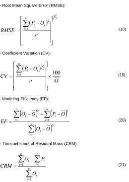
- Root Mean Square Error (RMSE):
21 1 2
n O P RMSE n i i i (18)- Coefficient Variation (CV):
O n O P CV n i i i 100 1 2 1
(19)
- Modeling Efficiency (EF):
n i i n i n i i i O O O P O O EF 1 2 1 1 2 2 (20)- The coefficient of Residual Mass (CRM):
n i i n i n i i i O P O CRM 11 1 (21)
Where the Pi is the estimated values, Oi is the measured values, n
is the number of samples and Ō is the average of the measured parameter. The minimum value of AE, RMSE, and CV is equal to zero, where the maximum value of EF is equal to one. Moreover, the EF and CRM can be a negative value. When the AE value is large, it means that the model acts in the worst case. The CV indicator illustrates the distribution ratio between estimated and measured values. The EF indicator compares the estimated values
with the average of measured values, where the negative value proves that the average value of measured data has a better assessment than estimated values. The CRM is an indicator of the tendency of the model to overestimate or underestimate. If the whole measured and estimated values are equal, then the value of RMSE, AE and CRM equals to zero and the value of CV and EF are equal to 100 and one respectively.
RESULTS AND DISCUSSION
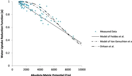
Figures 4 to 7 provides information on the coefficient of measured and estimated water uptake reduction by different models in different osmosis and matric potential levels. Generally, the results prove that the water uptake is a nonlinear reduction curve when the osmosis potential is constant and matric potential is reduced (e.g. Figure 4). In contrast, in a certain matric potential, the water uptake is declined by osmosis potential reduction (this is proved by the difference in the amount of maximum uptake coefficient in Figures 4 to 7). In addition, the water uptake reduction is intensified when the salinity and drought stresses happen simultaneously. This claim is proved by the difference of matric potential point where the plant is wilted; therefore, the plant is getting welted rapidly when the salinity and drought stresses are higher.
According to the statistical indicator, each model is ranked. To do this, first ranked model which the value of RMSE, AE, CV, and CRM are minimized or EF value is closed to one (Homaee et al., 2002; Loague and Green, 1991). When each statistical indicator is ranked, the average grade of each function is comprised of other functions. The calculated statistical parameters which are related to each water uptake reduction function and their ranking in each salinity level are presented in Tables 1 to 4.
Figure 4 depicts the fitting of different levels on measured data in the treatment of without salinity stress (salinity equal to 0.5 ds/m). The results of this Figure and Table 1 present when the plant just stays under drought stress, all of the simulated models have rather a good fitting by measured data. Moreover, this figure releases that in low moisture suction, the model of Feddes at al. (1976) has finer fitting compare to other models (Van Genuchten and Gupta, 1993; Dirksen et al., 1993). Table 1 indicates the appraisement of above model by statistical parameters which mean that the model of Feddes et al. has the first rank in fitting of measured data and model of Van Genuchten et al. and Dirksen et al. are placed in the next rankings.
Figure 5 shows the agreement of various models on measured data of salinity treatment of 5.5 ds/m and Table 2 indicates the evaluation of various models by calculated statistical parameters. These results prove that the water uptake reduction function in coincident stresses of salinity and drought in 5.5 ds/m can be an additive function, although the conceptual model of Homaee (1999) has a proper agreement, fairly.
Figure 4. Agreement of different models on measured data in the treatment of without salinity stress (0.5ds/m).
Figure 5. Agreement of different models on measured data in the treatment of 5.5 ds/m.
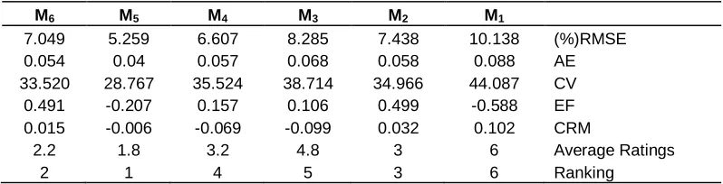
measured data of salinity treatment of 7.5 ds/m and Table 3 presents the evaluation of different models by calculated statistical parameters. The outcomes reveal
Figure 6. The agreement of different models on measured data of salinity treatment of 7.5 ds/m.
Figure 7. The agreement of different models on measured data of salinity treatment of 10 ds/m.
models, the model of Homaee (1999) and model of Skaggs et al. (2006) have proper fittings.
Table 1. Evaluation of different models by calculated statistical parameters of without salinity stress.
M9 M8 M7
14.260 14.203 13.622 (%)RMSE
0.059 0.055 0.055 AE
18.747 19.714 21.856 CV
0.409 0.451 0.459 EF
0.057 0.046 0.009 CRM
2.4 1.8 1.4 Average ratings
3 2 1 Ranking
M7: model of Feddes et al. (1978). M8: model of Van Genuchten et al.
(1984). M9: model of Dirksen et al. (1993).
Table 2. Evaluation of different models by calculated statistical parameters in treatment of 5.5 ds/m.
M6 M5 M4 M3 M2 M1
6.95 5.16 8.09 6.26 8.6 3.98 (%)RMSE
0.055 0.043 0.068 0.045 0.076 0.029 AE
29.036 26.257 32.254 25.717 35.208 21.392 CV
0.008 -0.046 -0.085 -0.048 0.055 0.004 EF
0.008 -0.046 -0.085 -0.049 0.055 0.004 CRM
3.2 2.8 5.4 3.4 4.8 1.4 Average Ratings
3 2 6 4 5 1 Ranking
M1: Additive model of Van Genuchten (1978). M2: Multiplicative model of Van Genuchten et al. (1987).
M3: model of Dirksen and Augustijn (1993). M4: Model of Van Dam et al. (1997). M5: Model of Homaee
(1999). M6: Model of Skaggs et al. (2006).
Table 3. The evaluation of different models by calculated statistical parameters of salinity treatment of 7.5 ds/m.
M6 M5 M4 M3 M2 M1
7.049 5.259 6.607 8.285 7.438 10.138 (%)RMSE
0.054 0.04 0.057 0.068 0.058 0.088 AE
33.520 28.767 35.524 38.714 34.966 44.087 CV
0.491 -0.207 0.157 0.106 0.499 -0.588 EF
0.015 -0.006 -0.069 -0.099 0.032 0.102 CRM
2.2 1.8 3.2 4.8 3 6 Average Ratings
2 1 4 5 3 6 Ranking
M1: Additive model of Van Genuchten (1978). M2: Multiplicative model of Van Genuchten et al. (1987). M3:
model of Dirksen and Augustijn (1993). M4: Model of Van Dam et al. (1997). M5: Model of Homaee (1999). M6:
Model of Skaggs et al. (2006).
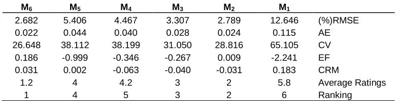
the agreement of different models on the mentioned salinity level and Table 4 proves the assessment of different models by calculated statistical parameters. The results describe that the reaction of Lolium perenne is a multiplicative when both salinity and drought happen at the same time where the model of Skaggs et al. (2006) and model of Van Genuchten (1987) have decent agreement among all models.
With the decrease of osmosis and matric potential, the
Table 4. The evaluation of different models by calculated statistical parameters of salinity treatment of 10 ds/m.
M6 M5 M4 M3 M2 M1
2.682 5.406 4.467 3.307 2.789 12.646 (%)RMSE
0.022 0.044 0.040 0.028 0.024 0.115 AE
26.648 38.112 38.199 31.050 28.816 65.105 CV
0.186 -0.999 -0.346 -0.267 0.009 -2.241 EF
0.031 0.002 -0.063 -0.040 -0.031 0.183 CRM
1.2 4 4.2 3 2 5.8 Average Ratings
1 4 5 3 2 6 Ranking
M1: Additive model of Van Genuchten (1978). M2: Multiplicative model of Van Genuchten et al. (1987). M3:
model of Dirksen and Augustijn (1993). M4: Model of Van Dam et al. (1997). M5: Model of Homaee (1999).
M6: Model of Skaggs et al. (2006).
decrease suction matric by 1 cm (Homaee et al., 2002). Hence, in a high level of salinity, the crop response to the salinity is a non-additive (Cardon and Letey, 1992). On the other side, in low salinity level, the crop response to simultaneous salinity and drought stresses is influenced by a combination of soil osmosis and matric potential. Therefore, the additive functions in low salinity condition have proper action (Skaggs et al., 2006). In comparison, by increasing the salinity level, the estimated transpiration with additive functions has a significant discrepancy with measured transpiration reduction (Cardon and Letey, 1992).
The negative value of CRM in models of M3, M4, and
M5 means that the water uptake amount calculates
overestimated while in M1 model, which is an additive
model, it calculates underestimated, in addition, the drought stress is more important rather than salinity stress. These results were proved by other researchers who worked on other crops such as Meiri and Shalhevet (1973) on reactions of Sepaskhah and Boersma (1979) on the dry weight of Wheat and Parra and Romero (1980) on the reaction of Bean.
CONCLUSION
According to the results, the amount of osmosis and matric potential are influenced by water uptake amount. When the osmosis potential is constant and matric potential is reduced, the water uptake amount is decreased. Furthermore, in a given matric potential, the water uptake is declined when the osmosis potential is reduced. When the plant was under drought stress only, the whole water uptake simulated models have a respectable agreement with measured data in drought stress condition. On the other hand, the reaction of Lolium perenne to coincident salinity and drought stresses is additive in low salinity level and it is multiplicative when the salinity degree is higher than 5.5 ds/m. Although the water uptake reduction of Lolium perenne is cumulative due to the existence of two
stresses simultaneously, the combined effect of salinity and drought stresses is fairly minus of aggregate effect of each stresses separately. Last but not least, among the multiplicative models, the model of Skaggs et al. (2006), Homaee (1999) and Van Genuchten (1987) show the proper agreement compare to other models.
ACKNOWLEDGEMENTS
We would like to express our deepest appreciation to all those who provided us the possibility to complete this dissertation. A special gratitude we give to our advisors, Dr. Davari and Dr. Banayan Aval, whose contribution in stimulating suggestions and encouragement, helped us to coordinate our project especially in experimental parts.
REFERENCES
Aronson LJ, Gold AJ, Hull RJ, 1987. Cool-season turfgrass responses to drought stress 1. Crop Sci, 27(6): 1261-1266.
Bresler E, McNeal BL, Carter DL, 1982. Saline and sodic soils: principles-dynamics-modeling (Vol. 10). Springer Science & Business Media.
Cardon GE, Letey J, 1992. Plant water uptake terms evaluated for soil water and solute movement models. Soil Sci Soc Am J, 56(6): 1876-1880.
Childs S, Hanks RJ, 1975. Model of soil salinity effects on crop growth 1. Soil Sci Soc Am J, 39(4): 617-622.
Denmead OT, Shaw RH, 1962. Availability of soil water to plants as affected by soil moisture content and meteorological conditions 1. Agron J, 54(5): 385-390.
Dirksen C, Augustijn DCM, 1988. Root water uptake function for nonuniform pressure and osmotic potentials. In Agronomy Abstracts (pp. 182-182).
Dirksen C, Kool JB, Korevaar P, Van Genuchten MT, 1993. HYSWASOR — Simulation Model of Hysteretic Water and Solute Transport in the Root Zone. In: Russo D., Dagan G. (eds) Water Flow and Solute Transport in Soils. Advanced Series in Agricultural Sciences, vol 20. Springer, Berlin, Heidelberg.
Feddes RA, Kowalik P, Kolinska-Malinka K, Zaradny H, 1976. Simulation of field water uptake by plants using a soil water dependent root extraction function. J Hydrol, 31(1-2): 13-26.
Gardner WR, 1960. Dynamic aspects of water availability to plants. Soil Sci, 89(2): 63-73.
Green SR, Kirkham MB, Clothier BE, 2006. Root uptake and transpiration: From measurements and models to sustainable irrigation. Agric Water Manag, 86(1-2): 165-176.
Hansen GK, 1974a. Resistance to water flow in soil and plants, plant water status, stomatal resistance and transpiration of Italian ryegrass, as influenced by transpiration demand and soil water depletion. Acta Agriculturae Scandinavica, 24(2): 83-92.
Hansen GK, 1974b. Resistance to water transport in soil and young wheat plants. Acta Agriculturae Scandinavica, 24(1): 37-48.
Herkelrath WN, Miller EE, Gardner WR, 1977. Water uptake by plants: II. The root contact model 1. Soil Sci Soc Am J, 41(6): 1039-1043. Homaee M, 1999. Root water uptake under non-uniform transient
salinity and water stress. Homaee.
Homaee M, Dirksen C, Feddes RA, 2002. Simulation of root water uptake: I. Non-uniform transient salinity using different macroscopic reduction functions. Agric Water Manag, 57(2): 89-109.
Loague K, Green RE, 1991. Statistical and graphical methods for evaluating solute transport models: overview and application. J Contaminant Hydrol, 7(1-2): 51-73.
Maas EV, Hoffman GJ, 1977. Crop salt tolerance–current assessment. J Irrigation Drainage Div, 103(2): 115-134.
Mathur S, Rao S, 1999. Modeling water uptake by plant roots. J Irrigation Drain Eng, 125(3), pp.159-165.
Meiri A, Shalhevet J, 1973. Pepper plant response to irrigation water quality and timing of leaching. In Physical Aspects of Soil Water and Salts in Ecosystems (pp. 421-429). Springer, Berlin, Heidelberg. Molz FJ, Remson I, 1970. Extraction term models of soil moisture use
by transpiring plants. Water Resour Res, 6(5): 1346-1356.
Molz FJ, Remson I, 1971. Application of an extraction-term model to the study of moisture flow to plant roots 1. Agron J, 63(1): 72-77. Nimah MN, Hanks RJ, 1973. Model for estimating soil water, plant, and
atmospheric interrelations: I. Description and sensitivity 1. Soil Sci Soc Am J, 37(4): 522-527.
Parra MA, Romero GC, 1980. On the dependence of salt tolerance of beans (Phaseolus vulgaris L.) on soil water matric potentials. Plant Soil, 56(1): 3-16.
Rowse HR, Stone DA, Gerwitz A, 1978. Simulation of the water distribution in soil. Plant Soil, 49(3): 533-550.
Sepaskhah AR, Boersma L, 1979. Shoot and root growth of wheat seedlings exposed to several levels of matric potential and NaCl-induced osmotic potential of soil water 1. Agron J, 71(5): 746-752.
Skaggs TH, van Genuchten MT, Shouse PJ, Poss JA, 2006. Macroscopic approaches to root water uptake as a function of water and salinity stress. Agric Water Manag, 86(1-2): 140-149.
Van Bavel CHM, Ahmed J, 1976. Dynamic simulation of water depletion in the root zone. Ecol Model, 2(3): 189-212.
Van Dam JC, Huygen J, Wesseling JG, Feddes RA, Kabat P, Van Walsum PEV, Groenendijk P, Van Diepen CA, 1997. Theory of SWAP version 2.0; Simulation of water flow, solute transport and plant growth in the soil-water-atmosphere-plant environment (No. 71). DLO Winand Staring Centre.
Van Genuchten MT, 1987. A numerical model for water and solute movement in and below the root zone. United States Department of Agriculture Agricultural Research Service US Salinity Laboratory. Van Genuchten MT, Gupta SK, 1993. A reassessment of the crop
tolerance response function. J Indian Soc Soil Sci, 41: 730-737. Van Genuchten MT, Hoffman GJ, 1984. Analysis of crop
production. Soil salinity under irrigation, pp. 258-271.
Whisler FD, Klute A, Millington RJ, 1968. Analysis of steady-state evapotranspiration from a soil column 1. Soil Sci Soc Am J, 32(2): 167-174.