A STATISTICAL MODEL FOR THE 2G, GSM COMMUNICATION SYSTEM IN UTTARAKHAND USING MULTIPLE REGRESSION TECHNIQUE

A STATISTICAL MODEL FOR THE 2G,

GSM COMMUNICATION SYSTEM IN

UTTARAKHAND USING MULTIPLE

REGRESSION TECHNIQUE

Professor, deptt of mathematics DIT, Dehradun [email protected]

Abstract

This paper introduces a statistical model by using the statistical methods in 2G,GSM communication system. Multiple regression formula is to calculate path loss. It is assumed that hb,W and α are three statistical variables. We use nakagami distribution to model hb,W and uniform distribution to model α.

Key Words- 2G, GSM, Multiple regression, nakagami distribution, uniform distribution.

1.Introduction

because the average rooftop level ,the road width and the road angle may be different. The statically approach [4] can solve above problem.

2. Formula description— a. Multiple regression formula—

Multiple regression formula [1] is described by the expanded sakagami formula [2]. The expanded sakagami formula is shown below by equation 1. Loss = 100 – 7.1 logW + 0.023 α +7.5 log hB - 24.37

3.7 log hb + 43.42 3.1 log d +20 log (f) ---(1)

Where

Loss= propagation loss [db]

d=distance between transmitter to receiver [m] W = road width [m]

α = road angle [deg]

= average building heiggt [m] = height of transmitter antenna [m] f= frequency [MHz]

= height of receiver antenna = 2 meter

Multiple regression formula is derived by [1] for urban areas and the formula is verified through a comparison with the simplified expanded sakagami formula shown by equation (1).

The frequency range of the regression formula is from 900 MHz to 1800 MHz. the distance range is 0.1 to 5 km. the range in the base station height is from 10m to 100m. The multiple regression equation is shown in equation (2).

Loss= 42 log(d) – 30 log (Hb) + 21 log (f) + 0.3 α – 0.003 α2 -9 log (w)-5 log _1.5 +54 ---(2)

In this regression formula hm is the height of receiver antenna. Other parameter definition is same as equation (1).

The path loss for the regression formula is shown in table 1 and fig.1 for W=9.1439, hB=8 mt, hb=24 mt,

Table-1

Distance(m) Path loss Path loss

α =45 α =90

500 200.45 195.72 1000 213.09 208.37 1500 220.49 215.76 2000 225.73 221.01 2500 229.80 225.08 3000 233.135 228.41 3500 235.94 231.22 4000 238.38 231.22 4500 240.53 235.80 5000 242.53 237.72

Fig.1 the variation of path loss as a function of d

b. the estimation of some parameters in regression formula—

the regression formula can predict the path loss for suburban areas on 2G frequency. In this study, the variation boundaries of three parameters are hB W and α evaluated at the same time. We assume that the parameters of hB

W and α are evaluated at the same time.We assume that the parameters of hB W and α in (2) are static. This

paper use nakagami distribution to model hB ,W and uniform distribution to model α The nakagami distribution

With shape parameter µ and scale parameter ω≥ 1, for x ≥ 1. If x has a nakagami distribution with parameters µ and ω, then x2 has a gamma distribution with shape parameter m and scale parameter ω_µ.

If µ= 1 , the nakagami distribution is reduced to Rayleigh distribution[6] whose probability density function is

Fx (x) = _ωe ω

If µ = 1 k _{2k 1} , the nakagami distribution reduced to Rice distribution whose PDF is [7]

Fx (x) = _ωe υ ω _I

o υ ω

Where Io(z) is the modified Bessel function of the first kind with order zero.

If µ →∞ , the Nakagami distribution is reduced to Gaussian distribution whose PDF is [8]

Fx (x) = _{√ π} e ω

3.The simulation result—

The path loss of the regression formula is simulated at the frequency of 900 MHz. In the simulation the average rooftop level hB, the road width W and the road angle α are modeled as random variable because these

parameters are not constancy at different areas.

There are two sets of parameter which are used in simulation. In fig.4 and fig.5

We calculate PDF and CDF for the path loss. We use the following distribution for hB W and α.

- Nakagami distribution function for hB with shape parameter µ→∞ and scale parameter ω=1.

- Nakagami distribution function for W with µ=1, ω=1.

- uniform distribution function for α with the range from 0 to 2π.

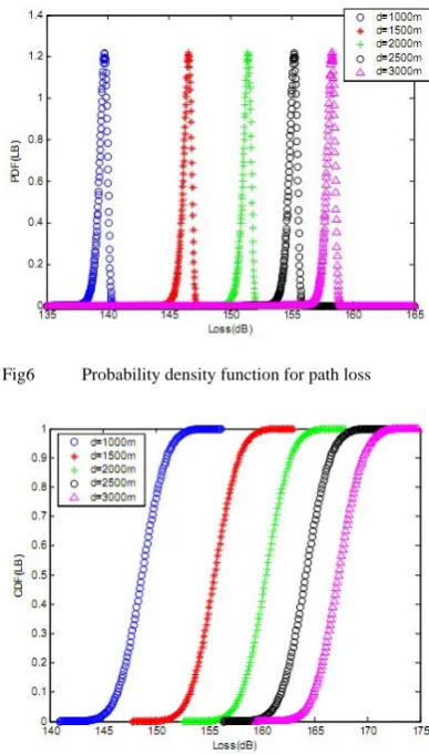
Fig 5 cumulative distribution function for path loss

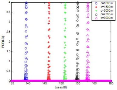
In fig.6 and fig.7 to calculate PDF and CDF for path loss we use

- Nakagami distribution function for hB with shape parameter µ=100 and scale parameter ω=3.

- Nakagami distribution function for W with µ→∞, ω=1. - uniform distribution function for α with the range from 0 to 2π.

The parameters hB W and α can choose other values according to the different circumstances.

Fig6 Probability density function for path loss

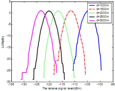
Apart from this we also calculate the other quantities which are required for error correction in digital communication system. These quantities are the level crossing rate and the average duration of fades.

For level crossing rate and average duration of fades it is assumed that the vehicle circles the base station at the rate of 36 km per hour. All three parameters , W and α are variables at the same time, where

- ,conforms to Nakagami distribution function with µ→∞ and W= 1.

- W confirms to Nakagami distribution function with µ = 1, ω = 1.

- α is modeled with the uniform distribution function with range from 0 to 2π.

Fig 8 and fig 9 show the level crossing rate and the average duration of fade of the regression formula.

Fig 8 level crossing rate

Fig 9 average duration of fade

IV. Conclusion-

statical analysis with the multiple regression formula. The model introduced in this paper is a useful tool for the design and analysis of data transmission scheme of the 2G mobile communication system.

REFERENCES

[1] KoshiroKITAO,ShinichiI Chitsubo.“Path Loss Prediction Formulain Urban Area for the Fourth-Generation Mobile CommunicationSystems”IEICETrans.Commun., Vol.e91-b, No.6, pp.0916-8516 2008.

[2] S.Sakagami,K,Kuboi,“MobilePropagation Loss Prediction forArbitrary Urban Environment”,IEICETrans.Commun.,Vol.J74-B-No.1,pp.17-25,Jan.1991.

[3] Jeonghoon Ahn,” Beyond Single Equation Regression Analysis: Path Analysis andMulti-Stage Regression Analysis” American Journal of Pharmaceutical Education Vol. 66, Spring 2002

[4] S.R.Saunders B.G.Evans. A physical-statistical model for land mobilesatellite propagation in built-upareas[J]. Proc.ICAP97 Edinburgh UK, 1997,:2.44-2.47.

[5] SaadAlAhmadi,Halim,Yanikomeroglu,“On the approximation of the generalized-k distribution by na gamma distribution for modeling composite fading channel”, IEEE Translation on wireless communications vol 9,issue 2, pages 706-713 ISSN: 1536-1276, 2010. [6] Karmeshu and Rajeev Aggarwal, “Efficiency of Rayleigh-inverse Gaussian distribution over k- distribution for wireless fading

channel”, volume 7 issue 1,page 1-7, 2006.

[7] Mohammad siraj and soumen kanrar, “Performance of modeling wireless network in realistic environment”, IJCN, Volume 2, Issue 1, 2010