https://doi.org/10.5194/amt-11-385-2018 © Author(s) 2018. This work is distributed under the Creative Commons Attribution 4.0 License.
GOCI Yonsei aerosol retrieval version 2 products: an improved
algorithm and error analysis with uncertainty estimation from
5-year validation over East Asia
Myungje Choi1, Jhoon Kim1,2, Jaehwa Lee3,4, Mijin Kim1, Young-Je Park5, Brent Holben4, Thomas F. Eck4,6, Zhengqiang Li7, and Chul H. Song8
1Department of Atmospheric Sciences, Yonsei University, Seoul, Republic of Korea 2Harvard-Smithsonian Center for Astrophysics, Cambridge, MA, USA
3Earth System Science Interdisciplinary Center, University of Maryland, College Park, MD, USA 4NASA Goddard Space Flight Center, Greenbelt, MD, USA
5Korea Ocean Satellite Center, Korea Institute of Ocean Science and Technology, Ansan, Republic of Korea 6Universities Space Research Association, Columbia, MD, USA
7State Environmental Protection Key Laboratory of Satellite Remote Sensing, Institute of Remote Sensing and Digital Earth,
Chinese Academy of Sciences, Beijing, China
8School of Environmental Science and Engineering, Gwangju Institute of Science and
Technology (GIST), Gwangju, Republic of Korea Correspondence:Jhoon Kim ([email protected]) Received: 17 July 2017 – Discussion started: 7 August 2017
Revised: 6 December 2017 – Accepted: 7 December 2017 – Published: 17 January 2018
Abstract. The Geostationary Ocean Color Imager (GOCI) Yonsei aerosol retrieval (YAER) version 1 algorithm was developed to retrieve hourly aerosol optical depth at 550 nm (AOD) and other subsidiary aerosol optical prop-erties over East Asia. The GOCI YAER AOD had accu-racy comparable to ground-based and other satellite-based observations but still had errors because of uncertainties in surface reflectance and simple cloud masking. In addi-tion, near-real-time (NRT) processing was not possible be-cause a monthly database for each year encompassing the day of retrieval was required for the determination of sur-face reflectance. This study describes the improved GOCI YAER algorithm version 2 (V2) for NRT processing with im-proved accuracy based on updates to the cloud-masking and surface-reflectance calculations using a multi-year Rayleigh-corrected reflectance and wind speed database, and inver-sion channels for surface conditions. The improved GOCI AODτG is closer to that of the Moderate Resolution
ing Spectroradiometer (MODIS) and Visible Infrared Imag-ing Radiometer Suite (VIIRS) AOD than was the case for AOD from the YAER V1 algorithm. The V2τGhas a lower
median bias and higher ratio within the MODIS expected
error range (0.60 for land and 0.71 for ocean) compared with V1 (0.49 for land and 0.62 for ocean) in a validation test against Aerosol Robotic Network (AERONET) AODτA
from 2011 to 2016. A validation using the Sun-Sky Radiome-ter Observation Network (SONET) over China shows similar results. The bias of error (τG−τA)is within−0.1 and 0.1,
and it is a function of AERONET AOD and Ångström expo-nent (AE), scattering angle, normalized difference vegetation index (NDVI), cloud fraction and homogeneity of retrieved AOD, and observation time, month, and year. In addition, the diagnostic and prognostic expected error (PEE) ofτGare
es-timated. The estimated PEE of GOCI V2 AOD is well corre-lated with the actual error over East Asia, and the GOCI V2 AOD over South Korea has a higher ratio within PEE than that over China and Japan.
1 Introduction
ab-sorbing solar radiance (aerosol–radiation interactions) and indirectly by altering cloud properties (aerosol–cloud inter-action; IPCC, 2013). Two aerosol optical properties (AOPs), the aerosol optical depth and single-scattering albedo, deter-mine the sign and magnitude of the shortwave aerosol ra-diative forcing of the atmosphere for different surface condi-tions (Takemura et al., 2002). Thus, accurate AOP retrievals are important for quantifying the role of aerosols in climate change. With respect to air pollution, ambient fine particu-late matter (PM) affects respiratory and pulmonary systems, resulting in an increased incidence of heart disease, strokes, and lung cancer (Lim et al., 2012). While PM information is often obtained from ground-based in situ measurements, the coverage of ground-based measurements is limited to the local scale and observational networks are often sparse, es-pecially in developing countries. However, satellite-based re-mote sensing can provide aerosol information over a much broader area. Chemical transport models (CTMs) make many assumptions in predictions of PM concentrations. Modeling accuracy can be improved significantly through data assim-ilation with satellite-retrieved aerosol optical depth (AOD) products (van Donkelaar et al., 2010).
East Asia has some of the highest aerosol concentrations in the world, with components that include desert dust, an-thropogenic carbonaceous aerosols, and sea salt (Kim et al., 2007; Yoon et al., 2014). Trends in aerosol concentrations in East Asia do not show the same significant decreases seen in Europe or North America (Zhang and Reid, 2010; Hsu et al., 2012), for reasons that are still unclear (IPCC, 2013).
The Geostationary Ocean Color Imager (GOCI), launched in 2010 as the first ocean color imager in geostationary or-bit (GEO), observes East Asia eight times per day from 00:30 to 07:30 Coordinated Universal Time (UTC; 09:30 to 16:30 Korea Standard Time (KST); Choi et al., 2012). Using the radiance measurements from eight spectral channels (412, 443, 490, 555, 660, 680, 745, and 865 nm) with high spa-tial resolution (500 m×500 m), the GOCI Yonsei aerosol re-trieval (YAER) version 1 (V1) algorithm was developed to retrieve hourly aerosol optical properties such as aerosol op-tical depth (AOD) with simple diagnostic parameters such as fine-mode fraction (FMF), Ångström exponent (AE), and single-scattering albedo (SSA; Choi et al., 2016). Because it has more channels with higher spatial resolution in the visi-ble and near-infrared (NIR) bands compared with recent and planned advanced meteorological sensors in GEO, including the Advanced Himawari Imager (AHI), the Advanced Base-line Imager (ABI), and the Advanced Meteorological Im-ager (AMI), GOCI provides valuable information related to AOPs. Hourly AOD from the GOCI YAER algorithm is in good agreement with Moderate Resolution Imaging Spectro-radiometer (MODIS) and Visible Infrared Imaging Radiome-ter Suite (VIIRS) AOD over East Asia (Xiao et al., 2016). The application of GOCI retrievals through data assimilation results in improved performance of several air quality fore-casting model predictions of AOD and PM concentrations
(Park et al., 2014; Saide et al., 2014; Jeon et al., 2016; Lee et al., 2016; Lee et al., 2017). For this reason, a need has arisen for GOCI aerosol retrievals with near-real-time (NRT) pro-cessing for operational air quality forecasting systems using data assimilation.
The lack of shortwave infrared (SWIR) channels in GOCI (similar to the 1.6 or 2.1 µm channels of MODIS) does not allow for the calculation of surface reflectance in the visi-ble range from top-of-atmosphere (TOA) reflectance in the SWIR range (Kaufman et al., 1997). Instead, the minimum reflectivity technique using the composite method (Herman and Celarier, 1997; Koelemeijer et al., 2003; Hsu et al., 2004) was applied in the GOCI YAER V1 algorithm. However, this methodology prevents the GOCI YAER V1 algorithm from being capable of near-real-time (NRT) processing because it required a monthly database for each year encompassing the day of retrieval for the determination of surface reflectance. In addition, the resulting retrievals have a slightly negative bias over land and a positive bias over ocean due to sur-face reflectance errors, compared with AERONET data dur-ing the Distributed Regional Aerosol Gridded Observation Networks – Northeast Asia 2012 campaign (DRAGON-NE Asia 2012 campaign; Choi et al., 2016).
In this study, version 2 (V2) of the algorithm is devel-oped to both allow NRT processing and improve accuracy. Monthly and hourly surface reflectance and wind speed de-terminations are modified using a climatological database from the multi-year GOCI dataset and reanalysis wind speed data, respectively. The surface reflectance database obtained from multi-year Rayleigh-corrected reflectance (RCR) sam-ples enables more accurate surface reflectance retrievals by increasing the availability of measurements that are not aerosol- or cloud-contaminated, compared with the 1-year samples of the V1 algorithm. The cloud masking and inver-sion spectral channels for aerosol retrievals were also modi-fied for better accuracy. Furthermore, retrieved GOCI YAER V2 AOD is evaluated using ground-based observation data, along with comparisons with both V1 and MODIS retrievals from March 2011 to February 2016, which is a longer eval-uation period than used in previous studies. The bias of the GOCI YAER V2 AOD is analyzed and uncertainties are es-timated to facilitate the application of GOCI AOD in data assimilation.
2 GOCI YAER V2 algorithm
2.1 Overview of the GOCI YAER V1 and V2 algorithm framework
A prototype of the GOCI YAER algorithm for use over the ocean (Lee et al., 2010) was developed using MODIS Level 1B (L1B) top-of-atmosphere (TOA) reflected radi-ance data and improved using nonspherical AOPs (Lee et al., 2012). Then, using real GOCI L1B TOA radiance data, the GOCI YAER V1 algorithm for use over land and ocean surfaces was developed (Choi et al., 2016). The algorithm is applied to cloud-free and snow/ice-free pix-els. Sets of 12 pixel×12 pixel blocks are aggregated to achieve 6 km×6 km spatial resolution and averaged after cloud/snow/ice masking and suitable pixel selection.
Unified aerosol models over land and ocean surfaces clas-sify aerosols using AOD at 550 nm, FMF at 550 nm, and SSA at 440 nm derived from the global Aerosol Robotic Network (AERONET) inversion database (Dubovik and King, 2000; Holben et al., 1998). This aerosol type classification (Lee et al., 2012) covers a range of AOPs: FMF from 0.1 to 1.0 at an interval of 0.1 and SSA from 0.85 to 1.00 at an interval of 0.05. A total of 26 aerosol models are assumed in the al-gorithm: nine highly absorbing, nine moderately absorbing, and eight nonabsorbing models. Note that AOPs to calcu-late AOD are constructed to account for hygroscopic growth and aggregation (Eck et al., 2003; Reid et al., 1998). Non-spherical properties are considered using the phase function derived from AERONET data.
Dark ocean surface reflectance is calculated using the Cox–Munk model (Cox and Munk, 1954) considering Fres-nel reflectance with a bidirectional reflectance distribution function according to geometry and wind speed in a precal-culated look-up table (LUT) with temporal interpolation of ECMWF wind speed data at 10 m above sea level (m a.s.l.) over dark ocean pixels (Dee et al., 2011). Land surface re-flectance is obtained using the minimum reflectivity tech-nique for each month, channel, and hour, and temporal in-terpolation is carried out over land, turbid ocean, and heavy aerosol pixels in the inversion step. In the algorithm, turbid water pixel detection is implemented using a difference of 660 nm TOA reflectance between directly observed and in-terpolated data from 412 and 865 nm (hereafter,1ρ660; Li et
al., 2003; Choi et al., 2016).
All eight channels are used over ocean surfaces, and differ-ent combinations of channels are used over land, depending on surface conditions. Measured spectral TOA reflectance can be converted to spectral AOD for all aerosol models us-ing the precalculated LUT, and spectral AOD can be con-verted to the corresponding value at 550 nm using the as-sumed AE of each aerosol model. Then, the mean value and standard deviation (SD) of AOD at 550 nm from dif-ferent channels are calculated for each aerosol model, and the three aerosol models with the lowest SD are selected.
The SD-weighted average of mean AOD at 550 nm from the three selected aerosol models is used as the AOD at 550 nm. An identical SD-weighted average is applied to the assumed AE, FMF, and SSA of the selected aerosol models to determine the final AE, FMF, and SSA values. This in-version method is focused primarily on the retrieval of AOD at 550 nm from multi-channel spectral information, and the AE, FMF, and SSA are determined from aerosol models se-lected for the best AOD fit. Thus, AOD at 550 nm is the main retrieval product, and the AE, FMF, and SSA are con-sidered as diagnostic parameters, or ancillary products. Note that the discrete ordinate radiative transfer (DISORT) code of the libRadtran software package is used to calculate TOA reflectance for the LUT construction based on scalar calcu-lations (i.e., intensity-only) and a plane-parallel atmosphere approximation (Mayer and Kylling, 2005).
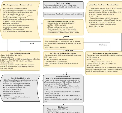
To improve the accuracy of AOP retrieval from GOCI measurements, AOD in particular, the new V2 algorithm is developed through piecewise upgrades to the V1 algorithm while retaining the structure and conceptual approach of the original algorithm. A flow chart of the GOCI YAER V2 algo-rithm is presented in Fig. 1. The improved parts of the V2 al-gorithm compared with V1 are the pixel masking and aggre-gation procedures, implementation of the climatological sur-face reflectance and wind speed from a 5-year climatological database for NRT calculations, turbid water detection, and in-version conditions for land, turbid water, and dark ocean pix-els. The aerosol model construction and inversion method for converting TOA reflectance to aerosol products are identical to those of V1. Details of the refined parts of the algorithm are introduced in the following subsections.
2.2 Pixel masking and aggregation procedure
Figure 1.Flow chart of the GOCI Yonsei aerosol retrieval version 2 algorithm. Yellow indicates improvements from version 1 to version 2, and gray indicates no change from version 1.
original 0.5 km×0.5 km L1B pixel resolution, aggregation from 0.5 km×0.5 km to 6 km×6 km resolution, and addi-tional masking at the 6 km×6 km resolution.
At the 0.5 km×0.5 km resolution, cloud masking over ocean surfaces is unchanged, but the land-surface cloud-masking steps are refined. The previous SD test of a 3 pixel×3 pixel block over land for identifying clouds and aerosols (Step 3 in Table 1, except for a threshold of 0.0025) works well for moderate- and high-AOD cases, but it over-masks heterogeneous surface reflectance pixels under low-AOD conditions. Thus, the threshold is relaxed to 0.015, and the mean-weighted SD test (Step 4 in Table 1) and the
ra-tio of maximum to minimum TOA reflectance at 412 nm within the 3 pixel×3 pixel grid are adopted (Step 2 in Ta-ble 1) as an alternative. To identify aerosols and clouds using a different technique, a pseudo Global Environment Monitor-ing Index (GEMI), developed by Pinty and Verstraete (1992) and Kopp et al. (2014) and applied in the operational VIIRS cloud-mask algorithm (Godin, 2014), is adopted (Step 6 in Table 1). The GEMI is based on the reflectance ratio between 865 and 660 nm and is defined as follows:
GEMI=G×(1.0−0.25×G)−100×Ref660−0.125 1.0−100×Ref660
Table 1.Cloud and other pixel masking steps of the GOCI YAER V2 algorithm.
Step Conditions Classification References
Masking at 0.5 km×0.5 km resolution
1 SD of TOA reflectance at 555 nm in 3 pixel×3 pixel blocks > 0.0025
Cloud over ocean (whole 9 pixels) Remer et al. (2005) Choi et al. (2016) 2 Ratio of maximum to minimum TOA
reflectance at 412 nm in 3 pixel×3 pixel blocks > 1.1
Cloud over land (whole 9 pixels) Hsu et al. (2013)
3 SD of TOA reflectance at 490 nm in 3 pixel×3 pixels block > 0.015
Cloud over land (whole 9 pixels) Wang et al. (2017)
4 Mean-weighted SD of TOA reflectance at 490 nm in 3 pixel×3 pixel blocks > 0.0025
Cloud over land (whole 9 pixels) Wang et al. (2017)
5 TOA reflectance at 490 nm > 0.4 Cloud over ocean and land Remer et al. (2005)
Choi et al. (2016)
6 Pseudo GEMI index < 1.87 Cloud over land Pinty and Verstraete (1992),
Kopp et al. (2014) 7 NDVI using TOA reflectance at 660 and
865 nm <−0.01
Inland water over land Hsu et al. (2013)
8 Ratio of TOA reflectance at 490 to 660 nm < 0.75,
and SD of TOA reflectance at 490 nm < 0.015 (or mean-weighted SD of TOA reflectance at 490 nm < 0.0025)
Homogenous dust call-back over land and ocean
Remer et al. (2005)
Aggregation to 6 km×6 km resolution
9 Number of available pixels after masking among 12 pixel×12 pixel blocks > 72
Discard darkest 20 % and brightest 40 % of pixels referred to TOA reflectance at 490 nm, and average remaining pixels
Remer et al. (2005) Levy et al. (2007) Choi et al. (2016)
Additional masking in 6 km×6 km resolution
10 SD of TOA reflectance at 412 nm > 0.003 and mean TOA reflectance at 412 nm in
12 pixel×12 pixel blocks > 0.22
Cloud over land and ocean
11 Mean TOA reflectance at 412 nm > 0.33 and mean TOA reflectance at 555 nm > 0.33
Cloud over land and ocean
12 Mean TOA reflectance at 412 nm < 0.30 and mean TOA reflectance at 660 nm > 0.2
Low aerosol signals and arid area masking
13 Difference in TOA reflectance at 660 nm between direct-measured value and linear-interpolated value from 412 and 865 nm <−0.01
Highly turbid pixel masking over ocean Li et al. (2003) Choi et al. (2016)
where
G=200×(Ref865−Ref660)+150×Ref865+50×Ref660 100×Ref865+100×Ref660+0.50
.
Note that Ref660and Ref865are the TOA reflectance at 660
and 865 nm, respectively. In addition, inland water pixels are filtered out using a normalized difference vegetation in-dex (NDVI) calculated using the TOA reflectance at 660 and 865 nm (Step 7 in Table 1). A dust call-back test used for ocean pixels is expanded to include both ocean and land pix-els and is coupled with a spatial homogeneity test (Step 8 in Table 1).
performed. A QA value of 0, 1, 2, or 3 for the V1 AOD was assigned for 6, 15, 22, or 36 remaining pixels, respec-tively. In addition, retrieved AOD values between−0.05 and 3.6 were assigned a QA value of 1, 2, or 3, and retrieved AOD values between −0.1 and−0.05 or between 3.6 and 5.0 were assigned a QA value of 0. The lower of these two QA values for each pixel was used as the final QA value. In the V2 algorithm, however, the retrieval is implemented if the number of remaining pixels is greater than 28, and the QA classification is eliminated. In addition, only pixels with retrieved AOD between−0.05 and 3.6 are included in the calculations. Small negative AOD values can be caused by surface reflectance errors in this algorithm. These are as-sumed to fall within the range of expected retrieval errors and are statistically significant under low-AOD conditions when compared with results from the MODIS DT algorithm (Levy et al., 2007, 2013). The threshold of maximum AOD of 3.6 is based on Lee et al. (2012), who considered the probability distribution of AOD in the region.
After the pixel aggregation procedure, merged TOA re-flectance at the 6 km×6 km resolution is filtered again. Bright and inhomogeneous pixels within a 12 pixel×12 pixel block are filtered using the mean and SD at 412 nm (Step 10 in Table 1), and pixels with high TOA reflectance at both 412 and 660 nm are also filtered out (Step 11 in Ta-ble 1). Furthermore, pixels with low atmospheric signal (dark at 412 nm) but high surface signal (bright at 660 nm), such as in arid areas, are also filtered out to avoid misidentification of the bright surface signal as aerosol (Step 12 in Table 1).
2.3 Climatological land surface reflectance database from multi-year samples
In the GOCI YAER algorithm, surface reflectance over land is handled differently to that over ocean. A minimum re-flectance technique to determine the surface rere-flectance from the composite Rayleigh-corrected reflectance (RCR) for each month and hour is applied over all land and turbid-water pix-els in the V1 algorithm. The GOCI YAER V1 algorithm was not capable of NRT processing because it required an adja-cent 2-month database encompassing the day of retrieval for the determination of surface reflectance.
To achieve NRT retrieval in the V2 algorithm, climato-logical land-surface reflectance for each channel, hour, and month are calculated over the 5-year period from March 2011 to February 2016. The V1 surface reflectance database was calculated at a 6 km×6 km resolution by the aggregation of 12 pixel×12 pixel data to extend the number of RCR sam-ples. The V1 surface reflectance calculation assumes that sur-face reflectance within a 6 km×6 km area is homogeneous. The V1 surface reflectance calculation resulted in slightly negatively biased AOD at low AOD over South Korea and Japan during spring 2012, which means that the surface re-flectance was overestimated (Choi et al., 2016). In the V2 al-gorithm, temporal RCR samples are expanded from a 1-year
period to a 5-year period, thereby improving performance under low aerosol conditions and reducing the negative bias in reflectance of the V1 algorithm. The spatial resolution of climatological land surface reflectance used in the V2 algo-rithm is 0.5 km×0.5 km for the L1B TOA reflectance, an improvement over the 6 km×6 km resolution used in the V1 algorithm. This higher resolution can capture highly spa-tially variable surface reflectance and improve the identical pixel matching between TOA and surface reflectance during pixel aggregation. The maximum number of composite 5-year RCR samples used to determine the surface reflectance of a single pixel is 155 (31 days×5 years). The darkest sam-ples (the lowest 0–1 % of the aggregate sample) are assumed to be cloud shadow and the brightest samples (3–100 % of the aggregate sample) are assumed to be affected by aerosols and/or clouds. Thus, the darkest 1–3 % of the RCR samples are averaged and used to determine surface reflectance, as in the V1 algorithm. According to Hsu et al. (2004), surface re-flectance can be obtained by finding the minimum RCR for each month, which corresponds to ∼3 % of the aggregate sample. The darkest 0–1 % of pixels are assumed, based on empirical grounds, to be cloud shadow and are thus excluded. This composite procedure is implemented for each month, hour, and channel. Monthly surface reflectance climatolog-ical data correspond to the middle of each month (day 15) and are linearly interpolated to the retrieval date. Major year-to-year land use changes over the 5-year period would result in an artificial AOD bias and should be addressed in future work.
2.4 Climatological ocean surface wind speed database from multi-year samples
To calculate dark ocean surface reflectance, the GOCI YAER V1 algorithm uses the ECMWF wind speed at 10 m a.s.l. from reanalysis data, which has a 6 h temporal resolution and 0.25◦×0.25◦spatial resolution. The ECMWF data are inter-polated to hourly resolution for use with observations. In the V2 algorithm, the wind speed from a 5-year average of cli-matological data is used. The wind speed from 5 years of data for each month, hour, and 0.25◦×0.25◦ area is aver-aged. This approach captures seasonal effects, such as higher (lower) wind speeds in winter (summer), and variations in the spatial distribution of wind speed, such as the higher (lower) wind speed in the open sea (coast). As in the land surface reflectance calculations, climatological wind speed data for each month correspond to the middle of each month (day 15) and are linearly interpolated to the retrieval date.
2.5 Refined pixel allocation for the land, turbid water, and dark ocean algorithms and
inversion conditions
pixels; the ocean algorithm is applied only over dark ocean surface pixels. A pixel with1ρ660 below−0.05 is assumed
to be dark ocean and is processed using the dark ocean al-gorithm. Pixels with 1ρ660 between−0.05 and−0.01 are
classified as turbid water and thus use the land algorithm. Pixels with 1ρ660 above −0.01 are assumed to be highly
turbid water and removed (Step 13 in Table 1). In some cases, ocean pixels have1ρ660above−0.05 with extremely
low TOA reflectance which could result from a combina-tion of low aerosol concentracombina-tions and dark ocean surface reflectance. Misidentification of these pixels as turbid water results in negative AOD over the dark ocean. Therefore, a threshold test to identify extremely dark ocean pixels using TOA reflectance at 660 nm is included in the V2 algorithm. The dark ocean algorithm is applied to pixels with1ρ660
be-tween−0.05 and−0.01 and TOA reflectance at 660 nm of below 0.07.
The channels selected for the inversion from measured re-flectance to aerosol optical properties are different for land, turbid water, and dark ocean pixels. In the V1 algorithm, the land and turbid water pixels use channels between 412 and 680 nm with surface reflectance less than 0.15, and the dark ocean pixels use all eight channels. In the V2 algorithm, the channels used for land pixels are the same as in the V1 al-gorithm, but the channels selected for turbid water and dark ocean pixels have been changed. In the atmospheric correc-tion for ocean color retrieval, the main assumpcorrec-tion is that water-leaving radiance is close to zero in the NIR range, and thus NIR bands are used for estimating aerosol loading in the atmosphere. The aerosol signal in the visible range is estimated from NIR measurements and the known relation-ships of aerosol signals in the visible and NIR range for var-ious aerosol types. Ocean color in the visible range is then retrieved after the atmospheric correction. When AOPs are the main retrieval target, however, water-leaving radiance is estimated as a climatological value or neglected. Both ap-proaches have limitations, as the accurate separation of ocean color and aerosol signals is difficult. Because water-leaving radiance is not considered in the current ocean surface re-flectance calculations of the GOCI YAER algorithm, chan-nels impacted by high water-leaving radiance are excluded in the V2 algorithm to minimize artifacts (Ahn et al., 2012). Thus, only two channels (412 and 865 nm) are used with the climatological surface reflectance database over turbid-water pixels, and four channels (412, 443, 745, and 865 nm) are used with the climatological surface wind speed database over dark ocean pixels.
2.6 Comparison of GOCI YAER V2 AOD with other data
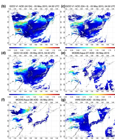
To evaluate the new masking techniques and climatological data used in the V2 algorithm, a retrieved dataset of GOCI YAER V2 AOD for 5 May 2015 is compared with that of the V1 algorithm under two scenarios: using all the quality
as-sured (all QA; QA=0, 1, 2, or 3) pixels and using only the highest quality assured (QA=3) pixels. The V2 products are also compared with MODIS/Aqua DT and DB, and VIIRS EDR products (Fig. 2). The overpass times of MODIS and VIIRS are generally near 04:00 UTC over the Korean Penin-sula, and thus GOCI 04:30 UTC results are selected for the comparison.
Most land pixels over the Korean Peninsula and Japan are not filtered out and are retrieved as low AOD in the DT, DB, and EDR algorithms. The DB algorithm retrieves high AOD over the bright surface of Manchuria located near 44◦N, 126◦E, but the DT and EDR do not retrieve AOD for those pixels because the algorithms are optimized for dark surface reflectance. The DT, DB, and EDR AOD are 0.7– 1.2 for land pixels over Hebei in China, located near 38◦N, 117◦E. Bright sun glint results in the masking of ocean pix-els over the Yellow Sea and East Sea for MODIS and VIIRS, respectively. The EDR algorithm captures an aerosol plume, resulting in AODs of ∼0.8 over the northern Yellow Sea, which is not captured by the DT algorithm, and the DT algo-rithm captures an aerosol plume resulting in AODs of∼0.6 over the East Sea close to Hokkaido, Japan, which is missed by the EDR algorithm.
The all QA GOCI V1 predicts low AOD in Korean Penin-sula and Japan areas, but cloud contamination results in high and inhomogeneous AOD, especially near the edge of the cloud cover. Sun-glint-masked ocean pixels are located at lower latitudes for GOCI than for MODIS and VIIRS. Thus, aerosol plumes detected by MODIS and VIIRS are both de-tected by GOCI. Although the GOCI YAER algorithm tar-gets dark land surface reflectance pixels, as do MODIS DT and VIIRS EDR, the aerosol plume over bright land surfaces in Manchuria captured by the DB algorithm is also detected. However, whether these pixels are from cloud contamination, bright land surface reflectance, or high AOD cannot be deter-mined.
When only pixels with QA=3 are applied to the V1 algo-rithm, most high- and inhomogeneous-AOD pixels, typically caused by unfiltered cloud contamination, are removed, but low-AOD pixels over land in South Korea and Japan are also removed. There are two possible reasons for the extensive masking in V1 using only QA=3 pixels for the case of low AOD over land. The spatial inhomogeneity test of the V1 al-gorithm is a simple SD of 3 pixel×3 pixel TOA reflectance with one fixed threshold, regardless of TOA reflectance. Al-though this approach works well in high-AOD cases, in low-AOD cases, inhomogeneous surface reflectance signals con-tribute to high SD and result in excessive masking. Another possible explanation is that these pixels have an AOD below −0.05 because of an overestimation of surface reflectance.
Figure 2. (a) GOCI RGB images and AOD for (b) GOCI V1 all QA, (c) GOCI V1 QA3, (d) GOCI V2, (e) MODIS/Aqua DT,
darker land surface reflectance is obtained from the clima-tological data, and this results in increased AOD compared with the large negative AODs seen from the V1 algorithm. Thus, fewer pixels are filtered out using the GOCI V2 algo-rithm and are retrieved as positive low AOD. The V2 AOD also shows fewer inhomogeneous features near the edges of clouds, similar to the MODIS and VIIRS AOD.
3 Long-term validation of GOCI YAER V2 AOD and AE
3.1 Ground-based measurements and ancillary satellite data
Two ground-based observation networks – the Aerosol Robotic Network (AERONET) and the Sun-Sky Radiome-ter Observation Network (SONET) – are used to quantify the accuracy of GOCI YAER V2 AOD (τG−V2)using data
from March 2011 to February 2016. AERONET is a ground-based aerosol remote sensing network of CIMEL sun-sky radiometer photometers maintained by the NASA Goddard Space Flight Center (Holben et al., 1998). Spectral AOD and AE are retrieved from direct solar irradiance measurements, and other optical/microphysical properties such as the vol-ume size distribution and refractive indices are retrieved from the inversion of spectral AOD with diffuse-sky radiance mea-surements. Uncertainties in AERONET AOD (τA)in the
vis-ible and NIR have been reported as±0.01 (Eck et al., 1999), which is much lower than is typical for satellite-retrieved AOD because of the minimal surface-reflectance effects in direct solar irradiance measurements and the highly accurate calibration. Thus, AERONET AOD is often used as the refer-ence dataset for satellite AOD validation. The fully calibrated and cloud-screened AERONET Version 2 Level 2.0 AOD at 550 nm and AE between 440 and 870 nm from direct mea-surements are used in this study (Smirnov et al., 2000). A total of 27 AERONET sites within the GOCI observation do-main, excluding specific short-period campaign sites, are se-lected for this analysis. Also, AERONET Version 2 Level 2.0 FMF at 550 nm and SSA at 440 nm from inversion products are used for the validation of GOCI FMF and SSA (Dubovik and King, 2000), The SONET is a ground-based aerosol re-mote sensing network of CIMEL sun-sky radiometers main-tained by the Institute of Remote Sensing and Digital Earth, Chinese Academy of Sciences (Li et al., 2015). The SONET also provides spectral AOD (τSONET)from direct sun
mea-surements and AE. A total of six SONET sites in China are selected for the validation of AOD at 550 nm.
In addition, the GOCI V1 AODs with all QA pixels (τG−V1allQA) and only pixels with QA=3 (τG−V1QA3) are
compared with V2 AODs to quantify improvements in the V2 algorithm. The MODIS DT AOD (τMDT)and DB AODs
(τMDB)of the highest quality pixels (QA=3) are also
com-pared over the same site and during the same period to verify
the GOCI AOD accuracy. Note that the VIIRS EDR AOD is used in the qualitative comparison in the previous section but is not included in the present validation because the VIIRS data are only available from January 2013.
3.2 Collocation criteria between ground- and satellite-based measurements
The comparison between satellite- and ground-based data is implemented with spatial and temporal collocation criteria. Hourly GOCI AOD pixels that are located within a 25 km radius of each ground site, and ground-based observation data within 30 min of each GOCI observation time, are av-eraged. The averages from both datasets are included if at least one measurement from each dataset is available. The collocation criteria used for the MODIS data are the same as for GOCI. After the collocation, 27 AERONET sites and 6 SONET sites are matched with GOCI land AOD obser-vations, and 17 AERONET sites are matched with GOCI ocean AOD observations. Note that the 27 AERONET sites matched with GOCI land AOD observations includes all 17 coastal AERONET sites matched with GOCI ocean AOD ob-servations because the coastal sites can be collocated with both land and ocean AOD measurements.
3.3 Statistical evaluation metrics
Following the method of Sayer et al. (2014), the statistical metrics for the evaluation contain the number of colloca-tion data (N); the Pearson’s linear correlation coefficient (R); the median bias (MB); the root mean square error (RMSE); andf, the fraction of data points within the expected er-ror range of the MODIS DT AOD (Collection 5), EEMDT=
±(0.05+0.15×τA), as described by Levy et al. (2007).
Each AOD product has an expected error range that can vary with the algorithm performance. To compare accuracies, the EEMDT is applied to all algorithms. Note that the expected
error range of the GOCI YAER V2 AOD (EEG_V2)is
esti-mated independently in Sect. 4.2.
3.4 Validation of GOCI YAER V2 land AOD and comparison with other data
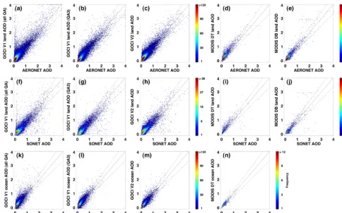
Results of a comparison between AERONET/SONET AOD and GOCI-retrieved AOD over land and ocean surfaces are presented in Fig. 3. Statistics from the comparison are sum-marized in Table 2. As seen in the qualitative comparison results (Fig. 2),τG_V1allQAshows many overestimated points
compared with τA because of remaining cloud
contamina-tion. About 20 % of pixels are filtered out with the QA=3 criteria (τG_V1QA3), and this results in a reduction of the
compari-Figure 3.Comparison of AOD between AERONET/SONET and GOCI/MODIS DT/MODIS DB over land and ocean surfaces. Thexaxis is land AERONET AOD, land SONET AOD, and ocean AERONET AOD from top to bottom, and theyaxis is GOCI YAER V1 for all QA, GOCI YAER V1 for QA=3, GOCI YAER V2, MODIS DT, and MODIS DB from left to right. Colored pixels represent a bin size of 0.02. Black dashed lines denote the one-to-one line, and dotted lines denote the expected error range of MODIS DT AOD.
Table 2.Statistics of land and ocean AOD comparisons between AERONET/SONET and satellite products, as shown in Fig. 3.
Satellite AOD algorithm N R MB f within EEDT RMSE
Land AOD comparison with AERONET
GOCI YAER V1 all QA 47 850 0.86 −0.015 0.49 0.24
GOCI YAER V1 QA3 38 183 0.92 −0.066 0.49 0.18
GOCI YAER V2 45 643 0.91 0.010 0.60 0.16
MODIS DT 3228 0.92 0.043 0.62 0.18
MODIS DB 3463 0.93 0.007 0.73 0.16
Land AOD comparison with SONET
GOCI YAER V1 all QA 12 974 0.83 −0.048 0.45 0.29
GOCI YAER V1 QA3 10 483 0.88 −0.103 0.42 0.27
GOCI YAER V2 12 238 0.86 −0.021 0.51 0.24
MODIS DT 733 0.82 0.104 0.46 0.29
MODIS DB 1258 0.86 0.000 0.67 0.27
Ocean AOD comparison with AERONET
GOCI YAER V1 all QA 19 945 0.83 0.056 0.55 0.17
GOCI YAER V1 QA3 18 308 0.88 0.043 0.62 0.13
GOCI YAER V2 18 499 0.89 0.008 0.71 0.11
son ofτG_V2withτAshow fewer overestimated points
com-pared with those ofτG_V1allQAbecause of the improved pixel
masking. This results in an increasedNandfwithin EEMDT
and decreased MB and RMSE compared withτG_V1QA3. The
increasedNcomes from the low-AOD points that are filtered out in τG_V1QA3. The number of underestimated points in
the low-AOD range decreased because of decreased surface reflectance using the 5-year samples. This results in lower bias (MB=0.010), decreased RMSE (0.16), and increased f within EEMDT (0.60). The R of 0.91 is similar to that
of τG_V1QA3(0.92). The N betweenτA andτG_V2 is about
14 times greater than the corresponding τMDT and τMDB,
mostly because of the hourly data available from GOCI com-pared with the twice-daily overpass data from MODIS. The spread of data points from MODIS and AERONET relative to the one-to-one line is lower than that from GOCI and AERONET, and this results in higherf within EEMDT( 0.62
for τMDT and 0.73 forτMDB). TheR and RMSE ofτMDT
andτMDBare similar to those ofτG_V2. The MB ofτMDBis
closest to zero, andτMDT has a positive MB of 0.043. The
overestimation ofτMDT has been attributed to the
urbaniza-tion effect of the biased reflectance estimaurbaniza-tion (Munchak et al., 2013) and has been corrected in the MODIS DT research algorithm (not used here) using the modified urban surface-reflectance algorithm (Gupta et al., 2016).
The GOCI V2 land AOD results can be recategorized as coastal or inland according to whether each site is collo-cated with both GOCI ocean and land AOD or with GOCI land AOD only. Mean AERONET AODs from coastal sites are lower (0.28) than those from inland sites (0.42). The intercomparison between coastal-site AERONET AOD and GOCI V2 land AOD has anRof 0.83, RMSE of 0.144, MB of −0.004, and f within EEMDT of 0.60. Results from
in-land sites have higherR(0.93), RMSE (0.171), MB (0.023), and the samef within EEMDT(0.60). High AOD is detected
more frequently at inland sites than at coastal sites.
A comparison between SONET AOD and satellite-retrieved AOD over land reveals thatτG_V2has higher
accu-racy thanτG_V1QA3, except in terms ofR. The reason for the
decreased accuracy inRofτG_V2may be the use of the same
climatological surface reflectance for each year, whereas in reality the surface reflectance changes annually. The τMDB
has the lowest MB and RMSE and highestf within EEMDT.
TheτMDThas a positive MB of 0.104.
In conclusion, most statistical parameters indicate that land τG_V2 accuracy is improved relative toτG_V1QA3 and
is comparable toτMDTandτMDB.
3.5 Validation of GOCI YAER V2 ocean AOD and comparison with other data
The changes of the GOCI YAER algorithm over ocean sur-faces between V1 and V2 include the cloud-masking tech-niques, the use of climatological wind speed data instead of each date data, pixel classification thresholds, criteria for
Figure 4. Relative frequency histograms of retrieved AOD from AERONET and satellites over(a)land and(b)ocean surfaces.
turbid-water and dark-ocean algorithm selection, and the choice of spectral channels. Results from the comparison of τG_V1QA3withτG_V1allQAshow decreasedN and RMSE, an
MB closer to zero,and increased R andf within EEMDT,
which is similar to the results over land sites except for MB. The refinement of the ocean algorithm from V1 to V2 results in improvement in most statistical parameters: decreased MB from 0.043 to 0.008, increasedf within EEMDT from 0.62
to 0.71, and decreased RMSE from 0.13 to 0.11. An MB closer to zero means that the modified channel selection in the turbid-water and dark-ocean algorithms, to avoid the ef-fect of water-leaving radiance variation, works efef-fectively. TheN between AERONET and GOCI V2 AOD over ocean surfaces is about 27 times greater than that for MODIS DT AOD, which is greater than that seen in the land compar-ison despite the same difference in observation frequency. The reason for this result is that most turbid-water pixels near the coast are filtered out in the MODIS DT algorithm, but are included in the GOCI YAER algorithm. Compared with the ocean τMDT, the ocean τG_V2 has slightly higher
RMSE, an MB closer to zero, slightly higherR, and slightly lowerf within EEMDT. In conclusion, most statistical
pa-rameters show that oceanτG_V2accuracy is improved
rela-tive toτG_V1QA3and is comparable withτMDT.
3.6 Comparison of AOD histogram distribution In Fig. 4, mean relative frequency histograms for landτA,
τMDTandτMDBmode of 0.1 reported by Sayer et al. (2013).
The landτG_V1QA3mode is 0.02 and those ofτG_V2,τMDT,
andτMDB are 0.12, 0.10, and 0.13, respectively, which are
similar to that of τA. Improvement in the land surface
re-flectance in V2 results in a reduced difference in mode be-tween AERONET and GOCI. The shape of the histogram of τMDBis better matched to that ofτAin the AOD range 0.05–
0.30 than toτMDTandτG_V2. The land-targeted histograms
of τMDT andτG_V2 have a similar shape to each other. The
two histograms have lower frequency modes and higher fre-quency AOD between 0.3 and 0.7 compared with τA. The τG_V2has a smoother shape due to a larger number of
coin-cident data points.
The mean relative frequency histograms forτA, collocated
with GOCI and MODIS ocean AODs, have a mode of 0.11, and those of oceanτG_V1QA3andτMDThave modes of 0.14
and 0.16, respectively. However, oceanτG_V2has a mode of
0.10, which is closer to that ofτAthan those ofτG_V1QA3and τMDT. Although the mode of oceanτMDTis higher than that
of τA, the magnitude of the peak is similar. The histogram
distributions of oceanτG_V1QA3andτG_V2have lower
mag-nitude peaks and more gradual decreases with increasing AOD compared toτA.
3.7 Validation of GOCI YAER V2 AE, FMF, and SSA over ocean and land surfaces
The AE intercomparisons between AERONET and GOCI YAER V2 over ocean and land surfaces are presented in Fig. 5a and b. Only AERONET AOD > 0.3 values are in-cluded because large errors exist in AE, due to surface re-flectance errors when AOD is low. Note that the GOCI AE is derived from the predefined values of the selected aerosol model, not from the retrieved spectral AOD. Compared with the V1 AE accuracy during the DRAGON-NE Asia 2012 campaign described by Choi et al. (2016; R=0.678 over both land and ocean surfaces), the V2 land and ocean AE have lower linear correlations with AERONET (R=0.505 and 0.459, respectively) from the 5-year validation. The DRAGON-NE Asia 2012 campaign was conducted in spring (March–May) when long-range transport of yellow dust from the Gobi and Taklamakan deserts in Asia, which has low AE with high AOD, is more frequent. Aerosol plumes with low AE and high AOD can be retrieved with higher accuracy compared with the generally low-AOD cases during other seasons. Thus, AE shows stronger linear correlation in spring (R of 0.63 over land and 0.57 over ocean) but is lower for other seasons (R of 0.24 over land and 0.22 over ocean). The highest frequency of points is close to the one-to-one line, but there is a significant discrepancy when AERONET AE is ∼1.3 but GOCI AE is∼0.6, particularly over land. This could be caused by varying surface reflectance errors for each channel or perhaps by a local-minimum problem in-duced from the LUT approach used for inverse modeling.
The FMF intercomparisons between AERONET inver-sion data and GOCI YAER V2 are similar to those of AE, as shown in Fig. 5c and d. This comparison also includes only AERONET AOD > 0.3 data. AERONET inversion products are retrieved from almucantar measurements, which are pos-sible when the solar zenith angle is greater than 50◦(Dubovik and King, 2000); thus, the number of points used in the com-parison are fewer than the AOD and AE from direct mea-surements. The correlation coefficients of FMF over ocean and land surfaces are similar to those of AE, as both param-eters are determined primarily by aerosol size.
The SSA intercomparisons between AERONET and GOCI YAER V2 have the lowest R (0.206 for land and 0.251 for ocean) among the products. The visible–NIR wave-length range is more sensitive to aerosol size than absorp-tivity. Thus, aerosol models are constructed more coarsely for SSA than for FMF, and the inversion methods focus on spectral matching of AOD at 550 nm, rather than on SSA-optimized retrieval, such as the OMI aerosol retrieval algo-rithm using ultraviolet radiation (Torres et al., 2013; Jeong et al., 2016). Nevertheless, the ratio of GOCI V2 SSA to AERONET SSA in a ±0.03 and±0.05 range is 47.7 and 68.0 % for land and 69.7 and 88.3 % for ocean, respectively, which is comparable to the OMI SSA presented by Jethva et al. (2014).
In conclusion, GOCI YAER V2 AE, FMF, and SSA com-pared with AERONET products are more biased and have lower correlation coefficients than seen for AOD. This indi-cates that the aerosol type selection is biased to coarse and nonabsorbing aerosols. To improve the accuracy of these pa-rameters, more accurate surface reflectance estimations and improved inversion methods are required.
4 Error analysis of GOCI YAER V2 AOD
Figure 5.Comparison between AERONET and GOCI YAER V2(a)land AE,(b)ocean AE,(c)land FMF,(d)ocean FMF,(e)land SSA, and
(f)ocean SSA. Note that collocated data are only for AERONET AOD > 0.3 for the AE and FMF comparisons, and AERONET AOD > 0.4 for the SSA comparison. Each colored pixel represents a bin size of 0.10 for AE, 0.05 for FMF, and 0.005 for SSA. Black dashed lines denote the one-to-one line, and blue dotted lines in the SSA comparison denote the±0.03 and±0.05 ranges.
4.1 Systematic bias analysis
4.1.1 Bias as a function of AERONET AOD
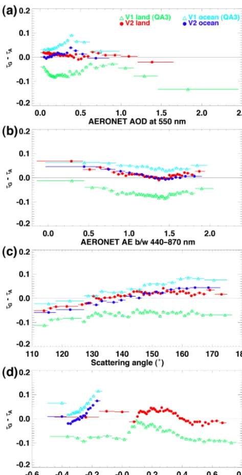
As shown in Fig. 6a, V1 land AOD has a negative bias in the low-AOD range because of an overestimation of sur-face reflectance. After implementing climatological sursur-face reflectance over land, the V2 land-AOD shows less bias than that of V1 and is close to 0 over the whole AOD range. This results from the increased probability of finding observation days with low aerosol loading using a 5-year dataset. The V2 ocean AOD shows a positive bias around 0.05–0.10 and high
Figure 6.Difference between GOCI and AERONET AOD in terms of(a)AERONET AOD,(b)AERONET AE,(c)scattering angle, and(d)GOCI NDVI. Each point represents the 50th percentile of 1000 collocated data points sorted in ascending order for eachxaxis value. The horizontal line through each point represents the range of collocated data points.
4.1.2 Bias as a function of AERONET AE
The V2 ocean and land AOD biases are close to zero when AERONET AE is within 1.3–1.6 and the accuracy of GOCI AE is high (Fig. 6b). However, these biases increase in the positive direction as AE deceases to 0.3 (large parti-cles). Compared with the biases of V1, those of V2 are re-duced for all AE ranges, but the pattern of difference in
AE remains. This could be due to errors in the assumed aerosol optical properties of extremely large particles. As-sumed aerosol models based on the global AERONET cli-matological database are categorized according to FMF and SSA, and the phase functions of nonspherical properties are averaged to one value for each model. In reality, various non-spherical shapes with the same FMF value may be present and may result in higher error at low values of AERONET AE. The differences may also be due to errors in aerosol type selection during the inversion process, as suggested by the decreased accuracy of low GOCI AE. Wavelength-dependent errors in calibration or surface reflectance assumptions may also contribute to the observed differences. Further investiga-tion is required to quantify the relative contribuinvestiga-tions of these errors.
4.1.3 Bias as a function of scattering angle
In Fig. 6c, the bias of ocean AOD changes from−0.05 to 0.10 as scattering angle increases from 110 to 175◦. The bias in land AOD shows a similar trend, but with a range of vari-ance from−0.05 to 0.05. As the scattering angle increases to 180◦, the atmospheric contribution to total TOA reflectance decreases compared with that from the surface because of the shorter light path length, which leads to an increase in AOD retrieval error (Sayer et al., 2013). This larger error at higher scattering angle is more distinct for ocean AOD than land AOD because of the difference in surface reflectance. The land algorithm performs characterization at each hour for surface reflectance using the composite method to reflect the BRDF effect. The ocean algorithm also considers geom-etry and wind speed in calculating the BRDF effect. How-ever, ocean bio-optical properties such as chlorophyll (Chl) or color-dissolved organic matter (CDOM) are not consid-ered in the current ocean surface reflectance calculation. This may be the cause of the relatively large error in ocean AOD compared with land AOD.
4.1.4 Bias as a function of NDVI
Figure 7.Difference between GOCI and AERONET AOD in terms of (a) GOCI cloud fraction within each aerosol product pixel (6 km×6 km),(b) the number of spatially collocated GOCI pix-els within a 25 km distance from AERONET sites, and(c)the spa-tial standard deviation of collocated GOCI AOD. The points, dotted lines, and horizontal lines in(a, c)are as defined in Fig. 6.
algorithm can still be slightly affected by these bio-optical ef-fects. Thus, positive biases persist for smaller negative NDVI values, which correspond to less turbid ocean pixels where ocean surface models that consider wind speed are utilized.
4.1.5 Bias as a function of cloud contamination
Despite applying several cloud-masking techniques, the re-maining cloud-contaminated pixels may still result in high positive biases in AOD. In this section, uncertainties due to cloud contamination are analyzed in terms of (1) cloud frac-tion at the aerosol product pixel resolufrac-tion (6 km×6 km), (2) the number of GOCI aerosol pixels collocated with each AERONET site, and (3) AOD spatial homogeneity.
First, the cloud fraction (CF) for one 6 km×6 km aerosol-product pixel can be calculated using the number of 0.5 km×0.5 km L1B pixels that remain after all masking
steps. In the aggregation step from the original L1B resolu-tion of 0.5 km×0.5 km to Level 2 aerosol-product resolution of 6 km×6 km, the maximum number of remaining pixels is 58 after performing all the individual masking processes and discarding the darkest 20 % and brightest 40 % of pix-els in a block of 12 pixpix-els×12 pixels (i.e., 144 pixels). The minimum number is set as 29, which corresponds to 50 % of the maximum value. If the number of remaining pixels is less than 29, then AOPs of that pixel are not retrieved. Note that pixels that are bright because of surface reflectance, not clouds, may be counted as a high CF, but it is difficult to completely distinguish these two cases at 500 m spatial res-olution. In Fig. 7a, the bias of ocean AOD is close to zero for a CF of 0.0, and increases to 0.1 as the CF increases to 0.5. The bias of land AOD is∼0.05 when the CF is close to zero, approaches to zero for 0.05 < CF < 0.25, and increases up to 0.05 as the CF goes to 0.4. This positive bias under high-CF conditions is similar to that of MODIS DT and DB AOD (Hyer et al., 2011; Shi et al., 2013). However, the pos-itive bias of land AOD at CF=0, which is not observed for MODIS DT and DB AOD, may be due to surface reflectance underestimations over bright surface in GOCI.
Next, the bias due to cloud contamination is analyzed with reference to the number of spatially collocated GOCI AOD pixels of each scene (NC)for each AERONET site location
(Fig. 7b). Because the GOCI AODs within a 25 km radius around each site are averaged if at least one pixel is available, NCcan indicate the existence of clouds near the AERONET
site over a broader domain. Note that the maximumNC of
ocean AOD pixels of 40 is less than that of land (56) be-cause ocean AOD is generally collocated with AERONET sites located on the coast. The bias of V2 land AOD is 0.1 for NC=1 and approaches zero asNCincreases. The V1 land
AOD had a negative bias, primarily because of surface re-flectance. Thus, the bias does not change withNC. The ocean
AOD bias is 0.05 forNC=1 and decreases for higherNC, up
to 30. However, high positive biases exist forNC> 30, which
could be due to problems in characterizing ocean surface re-flectance.
cloud contamination. Note that some recent aerosol retrieval algorithms have adopted a statistical spatial smoothness con-straint for AOPs in the inversion procedure to improve accu-racy (Dubovik et al., 2011; Xu et al., 2016).
In summary, the high cloud contamination in both each product-pixel (6 km×6 km) and neighboring pixel (within 25 km) domains results in high positive biases of up to 0.1. However, an independent analysis of the cloud-contamination-only effect is complicated by various factors including surface reflectance errors, resulting in a high bias under low cloud-contamination conditions.
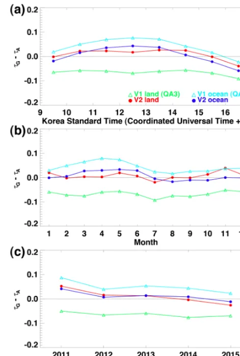
4.1.6 Bias as a function of hour, month, and year The GOCI AOD consists of eight hourly observations per day from 09:30 to 16:30 KST (centered time of each mea-surement), and the solar zenith and azimuth angle varies over a much wider range than that of low earth orbit (LEO) satellites. However, it requires more sophisticated treatments for properties such as surface reflectance, the aerosol phase function, and the calculation of Rayleigh scattering, which may result in accuracies that vary with measurement time. In Fig. 8a, the bias of land AOD decreases from about−0.1 for V1 to almost zero for V2, with no noticeable hourly depen-dence for V2. In contrast, the ocean AOD has a distinct di-urnal bias shape, which is close to zero at 09:30, 15:30, and 16:30 KST and ∼0.1 at 12:30 KST. This is consistent with the results of the bias analysis with reference to the scatter-ing angle.
The bias of land AOD as a function of month remains near zero (Fig. 8b). In contrast, that of ocean AOD increases up to 0.1 in spring (April–May) and to ∼0.05 in late fall and early winter (November–December), which can likely be at-tributed to monthly variations in Chl concentration over East Asia. The climatological Chl concentration reported by Ya-mada et al. (2004) is highest during spring (1.2–2.7 µg L−1), lower during late fall (0.8–1.2), and 0.2–0.4 µg L−1 during other seasons. Thus, the change in monthly bias for ocean AOD is likely affected by Chl concentrations in the current GOCI ocean AOD algorithm. The positive biases of the V1 ocean AOD during spring and late fall were reduced using V2 after changing the channel selection.
The V1 land AOD retrieved using monthly surface re-flectance data for each year shows a constant negative bias of about−0.05 from 2011 to 2015 (Fig. 8c). In contrast, the V2 land AOD retrieved using monthly climatological surface reflectance data from the 5-year dataset samples shows biases that are smaller than those of V1 but with increased variation. The increased variance for V2 could be due to a limitation of the application of climatological data, which cannot re-flect year-to-year changes in surface rere-flectance. The ocean AOD shows less variation in bias compared with the V2 land AOD, but it varies more than the V1 land AOD. This may be attributable to interannual variations in ocean surface re-flectance caused by ocean bio-optical properties.
Figure 8.Difference between GOCI and AERONET AOD in terms of local observation time, month, and year. The points are as defined in Fig. 7b.
Table 3.Expected errors of MODIS C6, VIIRS EDR, and GOCI over ocean and land.µ0andµare the cosine of solar zenith angle and satellite zenith angle, respectively.τAandτSare AERONET and satellite AOD, respectively.
Algorithm Diagnostic expected error (DEE) Prognostic expected error (PEE) Reference
Ocean
MODIS DT Linear regression with bias consideration:
−0.10τA−0.02 (lower bound) and 0.10τA+0.04 (upper bound)
Levy et al. (2013)
VIIRS EDR Linear regression with bias consideration:
−0.238τA+0.01 (lower bound) and 0.194τA+0.048 (upper bound)
Linear regression: ±(0.250τS+0.009)
Huang et al. (2016)
GOCI YAER V2 Linear regression: ±(0.185τA+0.037)
Linear regression: ±(0.206τS+0.030) Unique regression per AOD range: Table 4
This study
Land
MODIS DT Linear regression:±(0.15τA+0.05) Levy et al. (2010)
MODIS DB Linear regression:±(0.20τA+0.05) Linear regression with air mass factor consideration:
±(0.56+0.086)/(1/µ0+1/µ)
Sayer et al. (2013)
VIIRS EDR Linear regression with bias consideration:
−0.470τA−0.01 (lower bound) and−0.0058τA+0.09 (upper bound)
Linear regression: ±(0.34τS+0.023)
Huang et al. (2016)
GOCI YAER V2 Linear regression: ±(0.137τA+0.073)
Linear regression: ±(0.184τS+0.061) Unique regression per AOD range: Table 4
This study
of EE is that it increases linearly with AOD. Thus, a linear regression fit between the 68th percentile of absolute error and the reference AOD (AERONET or satellite AOD) is de-termined as EE. The 68th, 38th, and 95th percentile points correspond to 1, 0.5, and 2 SD intervals, respectively, assum-ing the error has a Gaussian distribution and no bias. Thus, 0.5 and 2 times the linear least square regression equation of the 68th percentile should correspond to the 38th and 95th percentiles, respectively. The EEs of MODIS, VIIRS, and GOCI AOD based on this approach are summarized in Ta-ble 3. Note that additional factors are considered in the EE calculations for each algorithm, such as bias information in MODIS DT over ocean surfaces and VIIRS EDR, and geo-metrical air mass factors in MODIS DB (Levy et al., 2013; Sayer et al., 2013; Huang et al., 2016).
To estimate DEE and PEE of the GOCI YAER V2 AOD using a linear least-squares regression equation, the abso-lute AOD difference between GOCI and AERONET is an-alyzed for AERONET and GOCI AOD in Fig. 9. The lin-ear DEE (0.185τA+0.037)and PEE (0.206τG+0.030)of
ocean AOD follow the 68th percentile points well (R=0.968
and 0.971, respectively). Doubled values of DEE and PEE for ocean AOD are well matched with the 95th percentile points. Although the linear DEE (0.137τA+0.073)and PEE
(0.184τG+0.061)of land AOD are well matched with the
68th percentile points (R=0.969 and 0.937, respectively), the PEE of land AOD includes discrepancies that vary over the AOD range. Significant discrepancies exist between the 95th percentile points and doubled values of the PEE of land AOD. Due to the existence of more complex error sources, the EE of land AOD cannot be accurately characterized in a linear relationship with AOD (Hyer et al., 2011). The es-timated linear DEE and PEE of land AOD show similar or lower slopes but higher offset compared with MODIS and VIIRS, which is assumed to be due to higher surface re-flectance bias in GOCI.
Figure 9.Absolute difference between GOCI YAER V2 AOD and AERONET AOD in terms of(a)AERONET ocean AOD,(b)AERONET land AOD,(c)GOCI YAER V2 ocean AOD, and(d)GOCI YAER V2 land AOD. The diamond, triangle, and square symbols represent the 38th, 68th, and 95th percentiles of 200 collocated data points sorted in ascending order ofxaxis value. In(a–d), the red line in each panel is the linear least-squares fit of the 68th percentiles, and the blue and green lines are half and double the red line values, respectively.
Table 4.Prognostic expected error (PEE) estimation of GOCI YAER V2 AOD according to the AOD range. The minimum PEE is labeled “noise floor”.
GOCI AOD range Ocean algorithm Land algorithm
“Noise floor” 0.044 0.048
−0.05≤τG<0.50 0.07−0.58τG+4.12τG28.81τG3+7.39τG41.50τG5 0.11−1.15τG+8.87τG225.05τG3+34.83τG418.93τG5
τG≥0.70 0.00+0.25τG 0.13+0.12τG
0.50≤τG<0.70 Highest between two fitting equations Highest between two fitting equations
The higher of these two computed values is applied when GOCI AOD is between 0.5 and 0.7. Both multiple PEEs show higher EE values near GOCI AOD of 0.1 (over ocean and land) and 0.6 (over land) compared with the linear PEEs, and thus they better match observations near the 68th percentile. The ratio of actual error to linear and multiple PEE follows the theoretical Gaussian distribution with a mean of zero and variance of 1 (N (0,1))as shown in Fig. 11, which is simi-lar to the results obtained for MODIS DB AOD (Sayer et al., 2013). Because the PEE of ocean AOD has a strong linear re-lation with GOCI AOD, there are fewer differences between linear and multiple PEE. However, the PEE of land AOD has a significantly different relationship with AOD, leading to differences in the distributions of linear and multiple PEE. Although the ratio betweenN (0,1)= −1 andN (0,1)= +1 (0.683) is closer to that of linear PEE for land AOD (0.680) than to the corresponding multiple PEE (0.669), the peak of N (0,1)is closer to that of multiple PEE than linear PEE. In addition, all linear and multiple PEEs of ocean and land AOD have slight positive biases compared withN (0,1).
Notwith-standing, the obtained PEEs of GOCI YAER V2 AOD, par-ticularly multiple PEE for land AOD, generally represent ac-tual errors well.
4.3 Regional performance
The obtained GOCI DEE and (multiple) PEE can be used for AOD validation for each site along with other statistical eval-uation metrics presented earlier. The validation results for all sites have been analyzed individually to compile the re-sults shown for each site, including the fraction of data points within DEE and (multiple) PEE. Spatial distributions of sta-tistical evaluation metrics are presented in Figs. 12 and 13 for land and ocean AOD, respectively.
improve-Figure 10.Absolute difference between GOCI YAER V2 AOD and AERONET AOD in terms of(a)GOCI YAER V2 ocean AOD and
(b)GOCI YAER V2 land AOD. The triangle symbols represent the 68th percentiles of 200 collocated data points sorted in ascending order ofxaxis value.
Figure 11.Comparison of observed(a)ocean and(b)land AOD error distributions with theoretical Gaussian distributions for the linear PEE (red) and multiple PEE (blue).
ment in V2 according to the statistical evaluation metrics and 6 sites have decreased accuracy in V2 compared with V1. In addition, the GOCI V2 land AOD shows less bias and has a higher fraction of data points within DEE and PEE over the Korean Peninsula compared with the Chinese and Japanese sites. The sites with the worst accuracy in V2 land AOD have a positively increased median bias. The reason for this de-crease in accuracy of some of the sites in V2 compared with V1 is likely the way that the surface reflectance database is constructed. Surface reflectance at the lower accuracy sites in V2, such as at Chiba University, Kobe, Xinglong, and Osaka, is brighter (urban surfaces) than at other sites, and the current identification threshold of the darkest 1–3 % of observations, without considering surface type, results in climatologically derived values for reflectance that are too dark at bright (ur-banized) surface sites. Tilstra et al. (2017) suggested that se-lecting the mode of the RCR histogram improves the charac-terization of surface reflectance of bright surfaces compared with selecting the minimum values of the RCR. Choosing different thresholds for various surface types may improve the accuracy of retrievals over sites that have high surface reflectance.
For ocean AOD, 14 sites show improvement in V2 and 3 sites have lower accuracy in V2 than V1 among the 17 coastal AERONET sites. In contrast to the increased median bias in land AOD, ocean AOD shows decreased median bias from V1 to V2. However, the lower accuracy sites do not differ significantly between V1 and V2 compared with land AOD. The fraction of data points within DEE and PEE for V1 ocean AOD at the Japan sites is higher than at the South Korean sites, but becomes similar in V2. The obtained DEE of V2 ocean AOD (94 %) is higher than the theoretical 1σ fraction (68 %). However, the PEE of V2 ocean AOD is 66 %, similar to the theoretical value. Thus, the obtained PEE can represent the error of GOCI AOD better than DEE.
5 Summary and outlook
Figure 12.Spatial distribution of statistical evaluation metrics for GOCI YAER V1 QA3 land AOD (first and third columns) and V2 land AOD (second and fourth columns). Left panels show mean AERONET AOD, correlation coefficient, and RMSE from top to bottom. Right panels show median bias, fraction within DEE, and fraction within multiple PEE from top to bottom.
and quantitatively analyzed uncertainties are highly suitable for use with air-quality monitoring and data assimilation in air-quality forecasting models, particularly when rapid diur-nal variations and transboundary transport are significant.
The objective of this study is the development of an im-proved GOCI YAER algorithm (V2) for NRT processing with higher accuracy. Cloud-masking procedures were re-vised to prevent false masking of low-AOD pixels over bright surfaces that was present in the previous version by adopt-ing recent MODIS and VIIRS cloud-maskadopt-ing methodology and improving existing V1 methodologies. To reduce the re-maining cloud and aerosol contamination effects in the sur-face reflectance database, the period of RCR samples is ex-panded from a 1-year to a 5-year period, to increase the prob-ability of finding cloudless low-AOD cases that improve the accuracy of the climatological surface reflectance database. In addition, the surface wind speed data are constructed as a climatological database for NRT retrieval without import-ing numerical weather forecast products. The GOCI spectral channel selection is revised to account for specific surface conditions: dark ocean, turbid water, and land surface. In
par-ticular, the channels from 500 to 700 nm, which are signifi-cantly affected by ocean bio-optical variations, are excluded from ocean AOD retrievals. As a result, the area of success-ful AOD retrieval and masking in the GOCI YAER V2 algo-rithm and the retrieved AOD values approach the results of MODIS and VIIRS AOD qualitatively, compared to that of GOCI YAER V1.
To confirm the improvements to GOCI AOD accuracy in V2, the retrieved GOCI AOD and MODIS AOD are com-pared with ground-based East Asia AERONET and China SONET measurements of AOD for 5 years from 1 March 2011 to 29 February 2016. The GOCI YAER land AOD shows a significant improvement from V1 to V2 with re-duced bias from about−0.07 to 0.01 and increasedf within EEMDTfrom 49 to 60 %. The comparison with SONET AOD
also shows improved results with reduced bias from about −0.10 to−0.02 and increasedf within EEMDT from 42 to
51 %. The GOCI YAER ocean AOD also shows reduced bias from about 0.04 to 0.01 and increasedf within EEMDTfrom
Figure 13.As for Fig. 12, except for GOCI ocean AOD.
V2 ocean and land AOD is more comparable to that of the MODIS DT and DB AOD products over East Asia.
Although retrieved GOCI YAER V2 AOD shows some bias with respect to AERONET AOD and AE, scattering angle, NDVI, cloud fraction and homogeneity of retrieved AOD, and observation time, month, and year, it never ex-ceeds an absolute value of∼0.1 for most variables. Account-ing for the observed increase in error with AOD, the intrinsic expected error of GOCI YAER V2 AOD was estimated using AERONET data. The linear DEE and PEE (0.185τA+0.037
and 0.206τG+0.030, respectively) for ocean AOD represent
the actual error well over the entire AOD range. The linear DEE of land AOD (0.137τA+0.073)also represents the
ac-tual error well. However, the acac-tual error does not increase linearly with GOCI land AOD; thus, the linear PEE of land AOD (0.184τG+0.061)shows variations over the AOD.
In-stead, the use of multiple PEE, which consists of PEE values for specific GOCI AOD ranges, improves the representation of the actual error.
Despite the algorithm improvements presented in this study, there is still potential for future improvements. The current version of the LUT was calculated using a scalar
ra-diative transfer calculation, which is less accurate for cal-culating Rayleigh scattering for short visible wavelengths (∼400 nm), and using a plane-parallel atmosphere approx-imation that is less accurate at high solar/sensor zenith angle. Vector radiative transfer calculations (i.e., consideration of polarization) and spherical-shell atmosphere approximations can calculate Rayleigh scattering at high accuracy and may improve the accuracy of the GOCI YAER algorithm. Also, recent statistically optimized aerosol retrieval algorithms uti-lizing the characteristics of spatial and temporal smoothness constraints for aerosols result in improved accuracy by in-creasing the aerosol signal (Dubovik et al., 2011; Xu et al., 2016). They also enable the simultaneous retrieval of mul-tiple geophysical variables, such as aerosol and surface re-flectance over land and aerosol and chlorophyll concentra-tions over the ocean, which can reduce the remaining error due to the predefined surface reflectance over ocean and land surfaces in the GOCI YAER algorithm.
re-trieval. Furthermore, GOCI-II will observe East Asia simul-taneously with the Geostationary Environmental Monitoring Spectrometer (GEMS) for trace gases (i.e., ozone, nitrogen dioxide, formaldehyde, and sulfur dioxide) and the AMI for meteorological parameters (i.e., cloud properties). Therefore, multi-sensor synergies contributing to a comprehensive un-derstanding of aerosols and trace gases, cloud, and ocean col-ors are expected.
Data availability. The GOCI L1B data are available on the home page of the Korean Institute of Ocean Science and Technol-ogy (KIOST) Korea Ocean Satellite Center (KOSC, 2018; http: //kosc.kiost.ac.kr/), and the GOCI YAER V2 aerosol data will be available at the same site. The GOCI YAER V2 aerosol data are also available through personal communication with the au-thors of the present paper. The AERONET data were obtained from https://aeronet.gsfc.nasa.gov (GSFC, 2018). The SONET data were obtained from http://www.sonet.ac.cn (SONET, 2018). The MODIS DT and DB aerosol data were obtained from https:// ladsweb.modaps.eosdis.nasa.gov (LAADS DAAC, 2018). The VI-IRS EDR aerosol data were obtained from https://www.class.ncdc. noaa.gov (NOAA, 2018). The libRadtran software package was obtained from http://www.libradtran.org (Mayer et al., 2017). The ECMWF wind speed reanalysis data were obtained from http:// apps.ecmwf.int/datasets (ECMWF, 2018).
Competing interests. The authors declare that they have no conflict of interest.
Acknowledgements. This work was funded by the Korea Mete-orological Administration Research and Development Program under grant KMIPA 2015-5010. This research was also supported by the “Development of the integrated data processing system for GOCI-II” funded by the Ministry of Ocean and Fisheries, South Korea. All principal investigators and their staff are thanked for establishing and maintaining the AERONET and SONET sites used in this investigation. The MODIS Dark Target, Deep Blue, and VIIRS aerosol teams are thanked for providing valuable data for this research. Jae-Hyun Ahn (KIOST KOSC) is thanked for preparing aerosol data distribution. Edward J. Hyer (US Naval Research Laboratory) and Andrew M. Sayer (USRA/GESTAR at NASA GSFC) are thanked for useful discussion of calculating uncertainties of satellite AOD. The editor and two anonymous reviewers are thanked for numerous useful comments, which improved the content and clarity of the manuscript.
Edited by: Alexander Kokhanovsky Reviewed by: three anonymous referees
References
Ahn, J. H., Park, Y. J., Ryu, J. H., Lee, B., and Oh, I. S.: Devel-opment of Atmospheric Correction Algorithm for Geostationary Ocean Color Imager (GOCI), Ocean Sci. J., 47, 247–259, 2012.
Choi, J. K., Park, Y. J., Ahn, J. H., Lim, H. S., Eom, J., and Ryu, J. H.: GOCI, the world’s first geostationary ocean color ob-servation satellite, for the monitoring of temporal variability in coastal water turbidity, J. Geophys. Res.-Oceans, 117, C09004, https://doi.org/10.1029/2012JC008046, 2012.
Choi, M., Kim, J., Lee, J., Kim, M., Park, Y.-J., Jeong, U., Kim, W., Hong, H., Holben, B., Eck, T. F., Song, C. H., Lim, J.-H., and Song, C.-K.: GOCI Yonsei Aerosol Retrieval (YAER) algorithm and validation during the DRAGON-NE Asia 2012 campaign, Atmos. Meas. Tech., 9, 1377–1398, https://doi.org/10.5194/amt-9-1377-2016, 2016.
Cox, C. and Munk, W.: Statistics of the sea surface derived from sun glitter, J. Mar. Res., 13, 198–227, 1954.
Dee, D. P., Uppala, S. M., Simmons, A. J., et al.: The ERA-Interim reanalysis: configuration and performance of the data assimila-tion system, Q. J. Roy. Meteor. Soc., 137, 553–597, 2011. Dubovik, O. and King, M. D.: A flexible inversion algorithm for
retrieval of aerosol optical properties from Sun and sky ra-diance measurements, J. Geophys. Res.-Atmos, 105, 20673– 20696, 2000.
Dubovik, O., Herman, M., Holdak, A., Lapyonok, T., Tanré, D., Deuzé, J. L., Ducos, F., Sinyuk, A., and Lopatin, A.: Statistically optimized inversion algorithm for enhanced re-trieval of aerosol properties from spectral multi-angle polari-metric satellite observations, Atmos. Meas. Tech., 4, 975–1018, https://doi.org/10.5194/amt-4-975-2011, 2011.
Eck, T. F., Holben, B. N., Reid, J. S., Dubovik, O., Smirnov, A., O’Neill, N. T., Slutsker, I., and Kinne, S.: Wavelength de-pendence of the optical depth of biomass burning, urban, and desert dust aerosols, J. Geophys. Res.-Atmos., 104, 31333– 31349, 1999.
Eck, T. F., Holben, B. N., Reid, J. S., O’Neill, N. T., Schafer, J. S., Dubovik, O., Smirnov, A., Yamasoe, M. A., and Artaxo, P.: High aerosol optical depth biomass burning events: A comparison of optical properties for different source regions, Geophys. Res. Lett., 30, 2035, https://doi.org/10.1029/2003GL017861, 2003. ECMWF: ECMWF wind speed reanalysis data, available at: http:
//apps.ecmwf.int/datasets, last access: 5 January 2018.
Godin, R.: Joint Polar Satellite System (JPSS) VIIRS Cloud Mask (VCM) Algorithm Theoretical Basis Document (ATBD), Joint Polar Satellite System (JPSS) Ground Project Code 474, 474-00033, GSFC JPSS CMO, 2014.
GSFC: AERONET data, available at: https://aeronet.gsfc.nasa.gov, last access: 5 January 2018.
Gupta, P., Levy, R. C., Mattoo, S., Remer, L. A., and Mun-chak, L. A.: A surface reflectance scheme for retrieving aerosol optical depth over urban surfaces in MODIS Dark Tar-get retrieval algorithm, Atmos. Meas. Tech., 9, 3293–3308, https://doi.org/10.5194/amt-9-3293-2016, 2016.
Herman, J. R. and Celarier, E. A.: Earth surface reflectivity cli-matology at 340–380 nm from TOMS data, J. Geophys. Res.-Atmos., 102, 28003–28011, 1997.