DETERMINATION OF BUFFER SIZE IN
SINGLE AND MULTI ROW FLEXIBLE
MANUFACTURING SYSTEMS
THROUGH SIMULATION
SRINIVAS.C
Assistant professor RVR & JC College of Engineering,
Guntur - 522 019, A.P., India
Dr.SATYANARAYANA B
Vice chancellor Andhra University,
Visakhapatnam - 530 003, A. P., India
DR.RAMJI K
Professor Andhra University,
Visakhapatnam - 530 003, A. P., India
Naveen Ravela,
Principal, 4
SCR Engineering College, Guntur - 522 619, A.P., India
Abstract
This paper presents the determination of buffer size for machines in single and multi row Flexible Manufacturing System (FMS) for the best layout obtained by genetic algorithm (GA) through simulation. To maximize the operating performance of FMS, many parameters must be considered, including the part types, sequencing, cost of transport between workstations, distance between machines and buffer sizes. Of the various critical factors, following three are considered for analysis: (1) minimizing the buffer size (2) minimizing the blocking and (3) maximizing the machine utilization. Simulation enables more efficient planning of the whole FMS, easy modifications before implementation on the real system. The software package FLEXSIM is used to develop the simulation model. A model of a optimum layout FMS obtained by GA that may contain a number of machines, input and output buffers, capturing part types flow quantities, part routes, from the database and AGV’s used as a means of transport, is built by FLEXSIM software. Analysis is done on the model to determine the optimum buffer size for the machines. Thus by performing simulation on the model optimum buffer size in the individual rows are established
1. Introduction
The purpose of this paper is to investigate and determine the buffer size of machines at the strategic level in rows. In particular, two commonly used row layouts single and multi rows are considered to assess the impact of automation and evaluate the effect of the buffer size on the total make span. Layout of flexible manufacturing system (FMS) involve distribution of different resources in a given FMS and achieving maximum efficiency of the services offered[3] With this in mind FMSs are designed to optimize production flow from the first stage as raw material to the finished product. The layout of the facilities has a direct impact on the production time and cost, especially in the case of large FMS For example Chiang and Kouvelis report that 30–70% of total manufacturing costs may be attributed to the layout and material handling[10]. Therefore, in the early stage of designing an FMS itself, it is necessary to have an idea of the layout of the machines and their buffer sizes.
Genetic Algorithms (GAs) are adaptive heuristic search algorithms premised on the evolutionary ideas of natural selection and genetics [11]. Gelenbe and Guennouni (1991) described a simulation tool called FLEXSIM for modeling FMS. FLEXSIM is designed to separate the specific FMS data from the simulation model to enhance the portability of the modeling tool [9].
A model is built by FLEXSIM for best layout which is obtained by GA. FMS performance is evaluated by measuring the make span for different buffer sizes for both the single and multi rows in order to determine the optimum buffer size in an FMS .Make span is influenced by order load and plant layout.. Production measures used for buffers evaluation include ([2,5]):
• Make span
• The average waiting time of ready parts which includes blocking. • Output queue length.
• Work in progress (WIP). • Machine utilization
A The simulation results demonstrate that substantial performance improvement can be achieved by finding the optimum buffer size and that the buffer size has an effect on performance. Thus by simulation optimum buffer size can be found out for optimum layout.
2. Problem of Arranging Work Stations into Rows
The manner of arranging of work stations largely depends on the type of production [3]. The work stations served by transporters are usually placed in one or multiple rows. An example of such placing is shown in Figure 1.
Fig1. Placing of workstations in multiple rows served by a transporter
In case of bad layout of work stations more transporters are required but they are under-utilized. Also the software for the control of transport is very complicated and it would be difficult to reach optimum states for the transporters. Therefore, it is of key importance how the work stations should be arranged in order to ensure optimum execution of transport of materials and work pieces. In principle, the work stations, fed by transporters, are arranged in one or multiple rows due to limited availability of the size and space of shop floor. Even when there are no space limitations, we need to know, into how many rows the work stations should be arranged so that the total material handling cost is kept to a minimum.
M3 M2
M1 M4 M5
M6
2. 1 Mathematical model of the machine layout problem
The objective of the machine layout problem is to minimise the total cost of transportation, incurred by all types of material handling devices present in the material handling system, put together.
The following assumptions are made during the process of modelling the single row FMS layout
• machines are arranged along a straight line • machines are oriented in only one direction • machines are rectangular with unequal sizes
• clearance between each pair of machines is variable
• distances between the machine are calculated with respect to their centroids
The machine layout problem can be formulated as follows:
Z = min C f L
where fij is the frequency of transport between the machines i and j, cij are the variable transport costs for the unit quantity which depends on the transport means used, must be known and Lij is the distance between the machines i and j. The number of all machines is equal to n. The costs of transport between two machines can be determined if their mutual distance Lij is known. During execution of the genetic algorithm, the values fij and cij do not change, the value Lij changes with respect to the mutual position of machines and with respect to position in the arrangement. In order to determine Lij we need also the dimensions of the machines, the minimum available distances between the machines, the widths of the transport paths and coordinate of the points of operating.
By using GA the optimum layout is obtained and the results are shown in table 2 and table 3 for single and multi row
3. Modelling and Simulation
Simulation involves the development of descriptive models of a system and exercising those models to predict the operational performance of the underlying system being modeled.
Discrete-event modelling and simulation is used for comparing alternatives in analysing, testing and design of FMS. Flexibility of the modelling approach is important, especially for comparisons of various policies.
The FMS studied is a layout with a bi-directional loop for the travel of the transporter. The FMS consists of 6 machine centers and 12 types of parts. The distance matrix, frequency matrix and the cost matrix are as shown below. The FMS system is shown in figure 3 for single row and figure 5 for multi row. The dimensions of the machines are shown in table 1.
0 40 80 21 62 90 0 4 4 6 4 5 0 1 1 1 2 1
40 0 72 12 24 28 4 0 2 5 2 3 1 0 1 1 1 1
fij= 80 72 0 14 41 9 Cij= 4 2 0 5 3 3 dij= 1 1 0 1 1 1
21 12 14 0 21 12 6 5 5 0 5 8 1 1 1 0 3 1
62 24 41 21 0 31 4 2 3 5 0 4 2 1 1 3 0 2
Table 1 Dimensions of work stations
Workstation Number Dimensions (length*breadth)
1 5.0*3.0
2 2.0*2.0
3 2.5*2.0
4 6.0*3.5
5 3.0*1.5
6 4.0*4.0
For the above problem the optimum and near optimum arrangement of machines obtained by applying GA [8] are shown in table 2 for single row FMS and table 3 for multi row FMS.
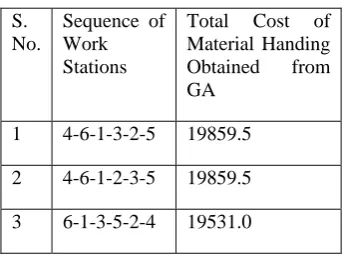
TABLE 2: Total Cost for Single Row FMS
S. No.
Sequence of Work Stations
Total Cost of Material Handing Obtained from GA
1 4-6-1-3-2-5 19859.5
2 4-6-1-2-3-5 19859.5
3 6-1-3-5-2-4 19531.0
TABLE 3 Total Cost for Multi-Row FMSTABLE 2
S. No. Sequence of Work Stations
Total Cost of Material Handing Obtained from GA
1 2-6-5-1-4-3 38615.5
2 2-5-1-6-3-4 33390.5
3 1-6-3-2-5-4 32058.5
12 21 31 28 24 14 41 9 72 90 62 21 80 40 1 6 5 4 3 2
Fig. 2 Network model showing work stations and the flow of work parts
Table 4 Details of parts entering at work station 1
Part Type Flow through work stations No. of Parts
1 1-2-4-6 12
2 1-2-6 28
3 1-6 90
4 1-4-5 21
5 1-3 80
6 1-5-6 31
7 1-5 31
Total 293
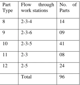
Table 5 Details of parts entering at work station 2
Part Type Flow through work stations No. of Parts
8 2-3-4 14
9 2-3-6 09
10 2-3-5 41
11 2-3 08
12 2-5 24
3.1Study Assumptions:
Prior to solving the problem we set certain assumptions that will be taken into account. These assumptions are:
• They are two sources, 6 machine centers with input and output buffers, 12 item types, transporters, and 4 sinks.
• All machines are of rectangular shapes,
• The machines are operated at the center of that space,
• All machines in the row look into the same direction as shown in Figure 1 • Processing times are constant value of 100.
• Loading and unloading times for the load are assumed to be 10 seconds each. These are commensurate with industry standards.
• Each job constitutes a unit load and mass is conserved during the network flow. This is a reasonable assumption as in a factory layout,
• The speed specifications of the AGV’s are pre-determined. We assume 2 m //sec. It is possible to change the speed using the operator controls.
• There are 6 control points on the transporter route. The transporter can be stopped at any control point and only at a control point. Most of these control points are designated pickup and delivery stations,. The above study assumptions also cover our input data. These assumptions and data are based on prior research that has been carried out in this field.
3.2. Building the Model
First the model of the layout is created using FLEX-SIM software [9]. The model is built taking into consideration and incorporating the inputs and assumptions made, so that it represents the real problem
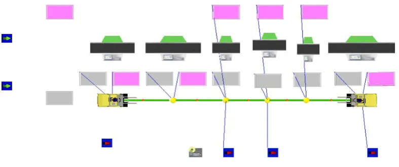
3.2.1.Single row:
The layout for single row is created as shown below and by clicking and dragging from the object library the objects such as queue, sink, source, processor, operator, nodes etc. the model is created. After building the whole layout make connections for each item type so that each item number follows its respective routes.
Fig 3: Optimum layout model for single row by GA
Fig 4: Optimum layout model for single row when simulation is performed
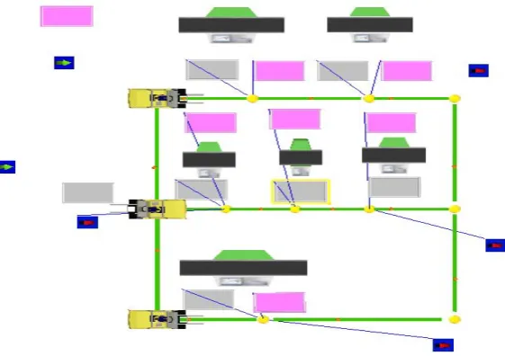
3.2.2. Multi-row:
For multi row, the maximum length of row (a), row height (r) and width of transport (w) are taken into consideration. The layout for multi row is created as shown below and by clicking and dragging from the object library the objects such as queue, sink, source, processor, operator, nodes etc. the model is created. After building the whole layout, make connections for each item type so that Each item number follow its respective routes.
Fig 6 Optimum layout model for multi row when simulation is performed
4. Results and Discussions
After identifying the optimal layout for the given input information both for the single and multi-row by GA. Analysis is done on the optimum layout to find the optimum buffer size for the machines in the optimum layout
For Single row optimum machine sequence obtained by GA: 6-1-3-5-2-4
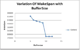
Table6 : Effect of Buffer size on Make span, Machine utilization, Blocking and Idleness of machines
S.NO BUFFERSIZE MAKESPAN MACHINEUTILISATION MACHINEIDLENESS MACHINE BLOCKING
1 5 35142.5 44.86 42.24 16.51
2 6 34042.5 46.32 37.67 16.09
3 7 33742.0 46.72 37.65 15.63
4 8 33542.5 47.01 37.57 15.42
5 9 33242.5 47.43 40.54 12.03
6 10 29442.5 53.55 46.45 0
7 11 29442.5 53.55 46.45 0
8 12 29442.5 53.55 46.45 0
Fig4 Variation of Make span with blocking for single row
Fig5 Variation of machine utiisation with Buffer size for single row
From the Table6, Fig3, Fig4 and Fig5 it can be easily observed that as the buffer size increases make span and blocking decreases while the machine utilization increases. Hence the optimum buffer size for the layout is 10 and minimum make span for single row is obtained as 29442.5.
For multi row optimum machine sequence obtained by GA : 1-6-3-2-5-4
Table7 Effect of Buffer size on Make span, Machine utilization, Blocking and Idleness of machines for Multi-row
S.NO BUFFERSIZE MAKESPAN MACHINEUTILISATION MACHINEIDLENESS MACHINE BLOCKING
4 4 36135.0 43.65 42.82 13.53
5 5 35537.5 44.22 42.74 13.04
6 6 35045.0 44.99 42.4 12.61
7 7 34052.5 46.29 41.61 12.10
8 8 33760.0 50.94 39.52 9.54
9 9 33467.5 51.45 39.44 9.11
10 10 29957.5 52.63 47.37 0
11 11 29957.5 52.63 47.37 0
Fig5 Variation of Make span with Buffer size for muti-row
Fig6. Variation of Machine utilisation with Buffer size for multi row
Fig7 Variation of Blocking with Buffer size for multi-row
5 Conclusion
In summary, this paper involves developing the model, simulating the optimum layout in single or multi rows in an FMS obtained by GA and an analysis is done on the layout to find out the optimum buffer size. One of the most important point we have found from this simulation is that the modeling and simulation can be used as a good tool for determination of optimum buffer size for machines in flexible manufacturing system.
Scope of future work:
After doing this project, we feel that the following points will be interesting topics for future study in this area: In future, there is a scope to include in the model by incorporating other criteria such as e.g., relations between the individual machines, shape of available area, I/O points, etc.
6. References
[1] Balic, J., (2001), Flexible Manufacturing Systems, DAAAM International, Vienna.
[2] Hamiani, A., Popescu, G.(1988): A knowledge-based expert system for site layout. In: Computing in Civil Engineering: Microcomputers to Supercomputers, pp. 248–256. ASCE, New York.
[3] Kusiak, A. (1990), Intelligent Manufacturing Systems. Prentice-Hall, New Jersey
[4] Goldberg, D.E. (1989) , Genetic algorithms. search, optimization and machine learning, Addison- Wesley [5] Banks, J., Carson ,J.S., Nelson, B.L. (1995). , Discrete-Event System Simulation, Prentice Hall Inc. [6] Pidd ,M. (1992). , Computer Simulation in Management Science, John Wiley & Sons Ltd.
[7] Pegden, C.D. , Shannon, R.E. , Sadowski ,R.P. (1990)., Introduction to Simulation Using SIMAN, Mc Graw-Hill Inc..
[8] A paper titled “a genetic algorithm approach for the design of single and multi-row flexible manufacturing systems “ published and presented at the 3rd international and 24th AIMTDR conference held at Andhra university, vizag during Dec13-15,2010. pp483-489
[9] Gelenbe, E. and Guennouni, H. (1991). “FLEXSIM: a flexible manufacturing system simulator.” European Journal of Operational Research (v53, n2), pp149-166.
[10] Kouvelis, P., and Chiang,W (1992)., A simulated annealing procedure for single row layout problems in Flexible manufacturing systems. International Journal of Production Research, 30 (4), 717- 732.