POWER CONSERVATION IN AD-HOC
NETWORKS USING DIJKSTRA’S
ALGORITHM & IDLE NODES
JACOB P CHERIAN ,
School of Computing Science & Engineering, VIT University, Vellore, TamilNadu-632014, INDIA
S M SULAIMAN ,
School of Computing Science & Engineering, VIT University, Vellore, TamilNadu-632014, INDIA
K MANIKANDAN ,
School of Computing Science & Engineering, VIT University, Vellore, TamilNadu-632014, INDIA
Abstract
The energy conservation in a wireless ad-hoc network is of great importance and significance. The nodes in a wireless environment are subject to less transmission capabilities and limited battery resources. The battery of node is energy limited and is not convenient to be replaced by the restriction of circumstance. But we have to ensure that even the slightest of energy is utilized and the overall power conserved in a wireless environment is greatly reduced. This paper aims at reducing the power conservation in a wireless ad-hoc network using Dijkstra’s algorithm and a set of available idle nodes.
Keywords: Wireless Ad-hoc Networks, Dijkstra’s Algorithm, Idle Nodes
1. Introduction
battery level and it may exclude from network path. After some time all the nodes may not be available during data transmission and the overall life time of the network may decrease.
2. Proposed Work
Wireless Ad hoc network is infrastructure less network. Communication in such type of network is either single hop or multi hop. A node can transmits or receive data to & from a node which lies in its vicinity. A node can transmit data to a longer distance if it has sufficient energy level. In wireless Ad hoc network a node is not only transmitting its own data but it also forward data of other nodes. [ Lindgren and Schelen,(2002)] .Resources available in scarce at a node may halt the data transmission either temporarily or permanently. All the nodes in the wireless Ad hoc network are battery operated and the life time of the network is depends upon the available battery power of a node . A node after data transmission may reach to a threshold level. If the battery power of a node reaches to threshold value, then node is not in position to either accept the data or send the data to other nodes in the network. It is known that the power required to transmit data from a source to destination node is directly proportional to the distance between the two nodes. Thus for a destination which is located far away from the source, direct transmission of data from source to destination will conserve a tremendous amount of source power. In such cases we have to find an optimal power conservation methodology which can solve this crisis. The power consumed for data transmission among the nodes is given by the formula :
ܧሺ݀ሻ ൌ ܽ݀ఈ ܿ (1)
Where a is a parameter related to the information, d is the distance between two nodes, constant c represents the energy consumption of information processing, and path loss index α relates to the propagation model, usually is set to 2 to 4. From equation 1 it is clear that as the value of ‘d’ i.e. the distance between the source and
destination increases, the power consumed will increase accordingly. It is also founded that if the number of nodes in between the source and destination are increased, they can be part of the communication between source and destination thus reducing the overall power required for transmission.
Proof:
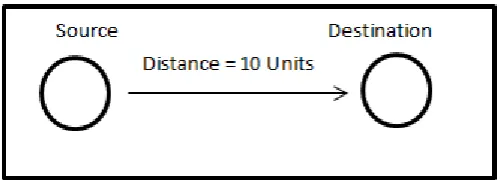
Let us consider the following two scenarios:
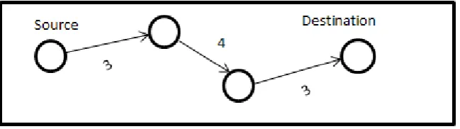
Figure 2: Transmission of data from source to destination via Intermediate Nodes.
Now, let us analyse the power consumed in both the cases. Let α =2 be the path loss index. Since we consider the same environment and the same information to be passed in both the scenarios, we can consider the values of a and c to be a constant (say k).In the first scenario the power consumed is E(d)= 102 + k units i.e 100 + k units. But in the second scenario it can easily be found that E(d) = (32 + 42 +32 )+ k units i.e 34 units. Thus it is evident that as the number of intermediate nodes increases, the power consumed at the source will be greatly reduced. It is also of interest that the maximum level of power conservation is achieved with a single intermediate node, if its placed exactly at the centre of the source and destination. But in actual scenario, all intermediate nodes may not satisfy this principle. Hence we use available intermediate nodes which form a shortest power consumed path with the source and the destination.
2.1 Shortest Power Consumed Path
A number of intermediate nodes may be available between a source and destination. But all of these nodes cannot be used for data transmission. Some nodes may be having very limited amount of power left, some nodes may be performing data transmission by itself and may not be currently available, while some nodes may be inactive [Banerjee and Misra,(2002)].. Hence a set of nodes should be selected such that they form a path from source to destination and this is the optimal power consumed path. There may be different paths which are available between the source and destination but all of them may not yield the shortest power consumption. Hence it is very important to identify the shortest power consumed path. In the proposed method, we find the shortest power consumed path using Dijkstra’s algorithm in which each edge represents the power required for data transmission among the respective nodes.
2.2 Dijkstra’s Algorithm
Let the node at which we are starting be called the initial node. Let the distance of node Y be the distance from the initial node to Y. Dijkstra's algorithm will assign some initial distance values and will try to improve them step by step.
1. Assign to every node a tentative distance value: set it to zero for our initial node and to infinity for all other nodes.
2. Mark all nodes unvisited. Set the initial node as current. Create a set of the unvisited nodes called the unvisited set consisting of all the nodes except the initial node.
3. For the current node, consider all of its unvisited neighbors and calculate their tentative distances. For example, if the current node A is marked with a tentative distance of 6, and the edge connecting it with a neighbor B has length 2, then the distance to B (through A) will be 6+2=8. If this distance is less than the previously recorded tentative distance of B, then overwrite that distance. Even though a neighbor has been examined, it is not marked as visited at this time, and it remains in the unvisited set. 4. When we are done considering all of the neighbors of the current node, mark the current node as visited
and remove it from the unvisited set. A visited node will never be checked again; its distance recorded now is final and minimal.
2.4 Sleep & Wake Up
Just like a semaphore in an operating system, the sleep and wakeup concept can be implemented in a wireless environment. Here we consider all nodes participating in data transmission to be currently active nodes. Once the data transmission is over, these nodes may not be having any functions to perform. So such nodes can go off to a sleep mode, where practically negligible power is consumed. Whenever, these nodes are identified to be a part of an optimal power consumed path, a wakeup signal can be send by the source node to make the node aware that it has to switch from inactive or sleeping mode to the active mode. However it should be ensured that all sleeping nodes are activated before the start of data transmission since sleeping nodes cannot receive any data or transmit them. Thus it may lead to loss of data. So such a situation should be avoided in prior to data transmission.
3. Proposed Algorithm
1. Find the distance between each pair of nodes in the network scenario and find the vicinity of each node. 2. Calculate the power required, E (d) for data transmission without intermediate nodes.
3.Using network topology find all the edges and vertices; Vertices are the wireless nodes, denoted by the set {V} and an edge eij is present if node ‘j’ is in the vicinity of node ‘i’, for all i, j ε {V}
4. Each edge is marked with the power required for data transmission between the vertices to which the edge belongs to.
5. Apply Dijkstra’s algorithm with ‘power’ as the matrix and find the minimal power consumed path from source to destination.
6. If there are any sleeping nodes in the path, send wakeup signals and alert them to be ready for data transmission
7. Remove any node from the optimal path if its current battery power is less than that required for transmission. 8. Once all nodes are ready, start data transmission.
9. After the entire data transmission, set all intermediate nodes to Sleep Mode.
4. Results & Analysis
Figure 3 : Graph showing the variation of power with increasing no:of nodes using proposed algorithm ( Without Considering Sleep & WakeUp)
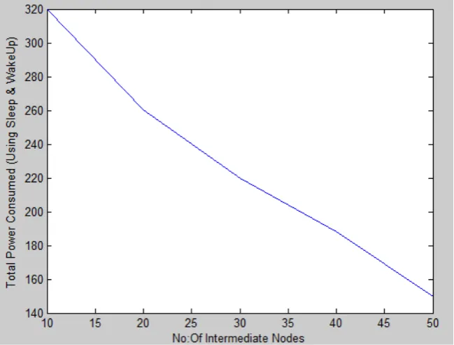
Figure 4 : Graph showing the variation of power with increasing no:of nodes using proposed algorithm considering Sleep & Wakeup concept
5.Conclusion
[6] Chen K, Xue Y, Shah SH, Nahrstedt K (2004). Understanding bandwidth-delay product in mobile ad hoc Networks. Comput. Commun., 27(10): 923-934.
[7] De Couto D, Aguayo D, Bicket J, Morris R (2003). A high-throughput path metric for multi-hop wireless routing. IEEE International Conference on Mobile Computing and Networking.