https://doi.org/10.5194/amt-11-5701-2018 © Author(s) 2018. This work is distributed under the Creative Commons Attribution 4.0 License.
Extinction and optical depth retrievals for CALIPSO’s
Version 4 data release
Stuart A. Young1, Mark A. Vaughan2, Anne Garnier1, Jason L. Tackett1, James D. Lambeth1, and Kathleen A. Powell2 1Science Systems and Applications, Inc. (SSAI), Hampton, VA 23666, USA
2NASA Langley Research Center, Hampton, VA 23681, USA
Correspondence:Stuart A. Young ([email protected]) Received: 5 June 2018 – Discussion started: 6 June 2018
Revised: 30 August 2018 – Accepted: 14 September 2018 – Published: 18 October 2018
Abstract. The Cloud–Aerosol Lidar with Orthogonal Po-larization (CALIOP) on board the Cloud–Aerosol Lidar In-frared Pathfinder Satellite Observations (CALIPSO) satellite has been making near-global height-resolved measurements of cloud and aerosol layers since mid-June 2006. Version 4.10 (V4) of the CALIOP data products, released in Novem-ber 2016, introduces extensive upgrades to the algorithms used to retrieve the spatial and optical properties of these lay-ers, and thus there are both obvious and subtle differences between V4 and previous data releases. This paper describes the improvements made to the extinction retrieval algorithms and illustrates the impacts of these changes on the extinction and optical depth estimates reported in the CALIPSO lidar level 2 data products. The lidar ratios for both aerosols and ice clouds are generally higher than in previous data releases, resulting in generally higher extinction coefficients and op-tical depths in V4. A newly implemented algorithm for re-trieving extinction coefficients in opaque layers is described and its impact examined. Precise lidar ratio estimates are also retrieved in these opaque layers. For semi-transparent cir-rus clouds, comparisons between CALIOP V4 optical depths and the optical depths reported by MODIS collection 6 show substantial improvements relative to earlier comparisons be-tween CALIOP version 3 and MODIS collection 5.
1 Introduction
The Cloud–Aerosol Lidar with Orthogonal Polarization (CALIOP) lidar (Hunt et al., 2009) on board the Cloud– Aerosol Lidar Infrared Pathfinder Satellite Observations (CALIPSO) satellite (Winker et al., 2010) has now acquired
over 12 years of global, height-resolved information on the location, extent, and optical properties of clouds and aerosols between the latitudes of 82◦S and 82◦N. The process of ex-tracting the desired optical and physical properties from the raw measurements is accomplished by a sophisticated suite of retrieval algorithms that performs a range of functions. These include calibration, determining the horizontal and vertical extent of atmospheric regions that contain particu-late (cloud or aerosol) matter, which we call features (Young and Vaughan, 2009, henceforth YV09), identifying the types of particles in those features, and retrieving profiles and layer integrals of the particulate backscatter and extinction in those features. An overview of the CALIOP processing algorithms has been provided by Winker et al. (2009).
of the feature two-way transmittance, which can be directly derived from CALIOP attenuated backscatter measurements made immediately above and below the boundaries of semi-transparent features (YV09). This procedure, already imple-mented in version 3 (V3), has been extended in V4. In the case of opaque layers, the initial lidar ratio in V4 is esti-mated from measurements rather than being assigned based on layer type, as was done in V3 (Sect. 2.2.3). This important change is paired with a totally new dedicated surface detec-tion algorithm (Vaughan et al., 2018b), which leads to a sig-nificantly more reliable identification of opaque layers than in V3. When the retrievals cannot be constrained or when the initial lidar ratio cannot be determined directly from the mea-surements, the extinction algorithm uses a set of initial lidar ratios, many of which have been significantly changed in V4. In addition to changes to the extinction retrieval algorithms and the analysis parameters, significant upgrades to preced-ing algorithms in the analysis chain also affect the retrieved quantities. For example, the new 532 nm nighttime calibra-tion algorithm (Kar et al., 2018) normalizes the measured at-tenuated backscatter profiles to a molecular model at higher altitudes than in the previous versions, in order to avoid errors caused by the presence of aerosols in the supposedly aerosol-free calibration region. This can lead to significant changes to the attenuated backscatter, particularly in the tropics, and would be expected, generally, to cause increases in the re-trieved optical quantities. The number and vertical and hori-zontal extent of the features subsequently detected have been impacted by changes in the calibration procedures (Kar et al., 2018; Getzewich et al., 2018) and the use of an improved molecular model (Kar et al., 2018). The retrieval of optical property profiles has also been affected by upgrades to the cloud–aerosol discrimination (CAD) algorithm (Liu et al., 2018). Large changes in calibration, especially at 1064 nm (Vaughan et al., 2018a), necessitated a complete restructur-ing of the probability density functions that drive the CAD algorithm, and hence the classification of features as clouds or aerosols is not uniformly consistent from V3 to V4. Addi-tionally, the generic stratospheric layer type identified in V3 has been eliminated in V4, and the CAD algorithm is now applied to all features detected in both the troposphere and the stratosphere. The algorithm that classifies clouds as wa-ter or ice has been refined in V4 (Avery et al., 2018). Simi-larly, the aerosol subtyping algorithms have been extensively revised, and the characteristic lidar ratios for several aerosol subtypes have been updated to reflect ongoing research car-ried out over the past decade. V4 now includes a new tro-pospheric aerosol subtype (dusty marine) and several strato-spheric aerosol subtypes (Kim et al., 2018).
Although changes to the algorithms that precede the tinction retrieval algorithm can be expected to impact the ex-tinction retrieval, this paper concentrates on the description of changes to the extinction algorithm and its associated anal-ysis parameters. Details of the extinction and optical depth
changes attributed to the upstream algorithms will be pub-lished separately (e.g., Kim et al., 2018).
The outline of this paper is as follows. Section 2 de-scribes changes to the extinction retrieval process, begin-ning with a description of changes to the analysis parame-ters (the lidar ratios and multiple scattering factors for clouds and aerosols), then proceeds to a description of changes to the various components of the actual extinction retrieval al-gorithm, which includes the description of a new algorithm for retrievals in opaque layers. Section 2 also describes re-vised algorithms for adjusting lidar ratios to achieve success-ful solutions, modification of lidar ratio uncertainties, and changes to the extinction quality control (QC) flags, which report the status of the extinction solution at the conclu-sion of the retrieval process. Section 3 presents the results of these changes and includes comparisons of the V4 and V3 retrievals in tropical clouds, lidar ratios retrieved in ice and water clouds using the new opaque layer algorithm, optical depths in opaque and semi-transparent clouds, and median profiles of extinction coefficient as a function of mid-cloud temperature and extinction QC value. We also provide ad-vice on the use of extinction QC values to filter data, and end with some general caveats regarding the retrieval of extinc-tion from elastic backscatter lidars. The mathematical details of the changes presented in Sect. 2 are described in the Sup-plement. This Supplement also includes descriptions of new criteria for determining the existence of solutions, an updated uncertainty analysis, a new initialization of the backscatter solution, and the initialization procedures for retrieving lidar ratios in opaque layers.
2 Changes in the retrieval process
The algorithms for retrieving profiles of particulate backscat-ter, extinction, and optical depth are described in YV09 and Young et al. (2013, 2016, henceforth Y1316). Changes and new features in the analysis parameters and in the algorithms used in the V4 retrievals have led to substantial improve-ments in these products when compared with those reported in V3. These changes are outlined in the following sections, with the mathematical details appearing in the Supplement. The most significant changes in the analysis parameters are to the initial estimates of particulate lidar ratios and their un-certainties for both aerosols and ice clouds (Sect. 2.1). The multiple scattering factors used for retrieving extinction pro-files in ice clouds and in opaque water clouds have also been changed.
value is close to the final value with the combined benefits of reliable and rapid convergence of the iteration. Further mod-ifications to the retrieval algorithms include changes to the assessment of what is and what is not a successful retrieval, and these are reflected in revisions to the extinction QC flags (Sect. 2.2.6).
2.1 Changes to the initial lidar ratios and multiple scattering factors
In this section we summarize the changes introduced in V4 to the initial lidar ratios for aerosols and clouds. These ini-tial values are used by the extinction retrieval algorithm for the analysis of semi-transparent layers where the retrievals cannot be constrained by an independent measurement of the effective two-way transmittance of the layer. The ef-fective, two-way layer transmittance,TP2, can be expressed as exp(−2ητP), where ητP is the effective particulate op-tical depth of the layer, τP is the single-scattering optical depth, and η is a layer-effective multiple scattering factor (0≤η≤1) that accounts for the apparent reduction in op-tical depth caused by the backscatter of multiply scattered photons into the receiver (Platt, 1973). The effective trans-mittance is biased high with respect to the single-scattering (η=1) value. The final values of the lidar ratios may be re-duced from the initial values if it is found that the initial val-ues are too large to permit a solution. For opaque layers, the initial lidar ratios are now derived from the measurements, as described in Sect. 2.2.3.
The relative uncertainties in the initial lidar ratios have also been changed in V4. In most cases these are consid-erably smaller than in V3. As the lidar ratio uncertainty is usually the dominant factor determining the overall uncer-tainties in the retrieved extinction data products, these latter uncertainties are expected to be smaller than in V3.
In addition to changes in the lidar ratios and their uncer-tainties, there are also changes to the multiple scattering fac-tors for clouds. Whereas these facfac-tors were constants in V3, in V4 they are now functions of cloud 532 nm attenuated backscatter centroid temperature for ice clouds (Garnier et al., 2015) and are obtained from 532 nm depolarization mea-surements for opaque water clouds (Hu, 2007).
2.1.1 Initial lidar ratios for aerosols
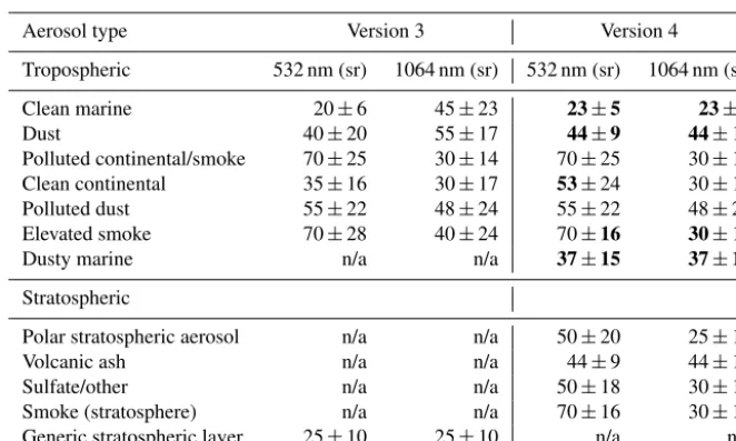
The initial lidar ratios and their uncertainties for several of the aerosol subtypes have been revised for V4 (Kim et al., 2018). As can be seen in Table 1, V4 specifies larger 532 nm lidar ratios for dust (by 10 %), clean marine (by 15 %), and clean continental (by 51 %) aerosols. These higher lidar ra-tios, which are consistent with improved knowledge gained over the past decade (e.g., Tesche et al., 2009; Nisantzi et al., 2015; Liu et al., 2015; Papagiannopoulos et al., 2016; Haarig et al., 2017), contribute to higher values in the re-trieved backscatter, extinction, and optical depths than were
reported in V3. Our better understanding of lidar ratio vari-ability led to significant reductions in the uncertainties as-cribed to the lidar ratios for marine, desert dust and smoke aerosols, resulting in generally lower uncertainties in the re-trieved products for these aerosol types. As explained in Kim et al. (2018) and documented in the V4 CALIPSO Data Products Catalog (Vaughan et al., 2018c), the nomencla-tures of the aerosol type 3 “polluted continental” and type 6 “smoke” were changed in version 4.1 to “polluted conti-nental/smoke” and “elevated smoke”, respectively. V4 also adds a new “dusty marine” tropospheric subtype and five new stratospheric subtypes. The lidar ratio for the dusty marine mixture is significantly higher than that for clean marine, but significantly lower than that for polluted dust. Aerosols iden-tified as dusty marine in V4 were generally classified as pol-luted dust in V3. Some aerosol lidar ratios at 1064 nm have also been changed, as shown in Table 1. Note that there was no cloud–aerosol classification in the stratosphere in V3 and that all stratospheric layers were assigned an initial lidar ratio of 25 sr and a multiple scattering factor of 1.
Combined with changes in the CAD and aerosol subtyp-ing algorithms that have led to changes in the identification of some aerosol types, these new lidar ratios yield extinction profiles and optical depths that can differ noticeably from those reported in V3. For aerosols, changes to optical depths and extinction profiles are largely the result of changes to the lidar ratios for the particular aerosol subtypes, and of changes in the algorithms that determine these subtypes, and are only rarely due to changes to the extinction algorithm. Therefore, changes in aerosol optical depths are discussed in a separate publication (Kim et al., 2018).
2.1.2 Multiple scattering factors and initial lidar ratios for clouds
Ice clouds
Table 1.Initial lidar ratios and their uncertainties, in units of steradians, that characterize each of the aerosol subtypes reported in V3 and V4. V4 values that have changed with respect to V3 are in bold text.
Aerosol type Version 3 Version 4
Tropospheric 532 nm (sr) 1064 nm (sr) 532 nm (sr) 1064 nm (sr)
Clean marine 20±6 45±23 23±5 23±5
Dust 40±20 55±17 44±9 44±13
Polluted continental/smoke 70±25 30±14 70±25 30±14
Clean continental 35±16 30±17 53±24 30±17
Polluted dust 55±22 48±24 55±22 48±24
Elevated smoke 70±28 40±24 70±16 30±18
Dusty marine n/a n/a 37±15 37±15
Stratospheric
Polar stratospheric aerosol n/a n/a 50±20 25±10
Volcanic ash n/a n/a 44±9 44±13
Sulfate/other n/a n/a 50±18 30±14
Smoke (stratosphere) n/a n/a 70±16 30±18
Generic stratospheric layer 25±10 25±10 n/a n/a
n/a: not applicable.
ητCALIOP) obtained from direct measurements of TCALIOP2 must be rescaled by a temperature-dependent multiple scat-tering factor to ensure the appropriate temperature-dependent correspondence between τCALIOP and τIIR. As shown in Fig. 1a, the V4 sigmoid approximation of η, which was re-trieved assuming that these clouds are composed of severely roughened aggregated columns (Yang et al., 2013), increases from a value of 0.46 at a centroid temperature of 0◦C to 0.79 at−90◦C.
As a consequence of the changes in theη parameteriza-tion, the initial lidar ratio estimates for ice clouds have also been changed. In V3 and earlier data releases, an initial lidar ratio of 25 sr was used in all ice cloud extinction retrievals. Comparisons of V3 optical depths for semi-transparent ice clouds with IIR absorption optical depths at 12.05 µm (Gar-nier et al., 2015) and a radiative closure experiment using MODIS 11 µm radiances by Holz et al. (2016) showed, on av-erage, quite good agreement for constrained retrievals. How-ever, for unconstrained retrievals, several studies of semi-transparent ice clouds showed that, when used in conjunction withη≈0.6, the initial lidar ratio of 25 sr was generally too small. Josset et al. (2012) found, from their analyses of op-tical depths determined from CALIOP and CloudSat echoes from the ocean’s surface, that the initial lidar ratio was about 25 % too low. Their analysis of semi-transparent cirrus pro-duced a mean multiple scattering factor of 0.61±0.15, with a corresponding mean lidar ratio of 33±5 sr that showed slight variations as a function of temperature and latitude. A sim-ilar conclusion was reached by Garnier et al. (2012), who compared CALIOP optical depths with those measured by the IIR at 12.05 µm and found that there was an inconsis-tency between CALIOP V3 constrained and unconstrained
optical depths, and that using a revised initial lidar ratio de-rived from constrained retrievals greatly improved the com-parisons. Holz et al. (2016) showed that the CALIOP uncon-strained optical depths were substantially smaller than the MODIS Collection 5 values. The authors showed that a much better agreement was achieved when CALIOP unconstrained retrievals using a lidar ratio of 32 sr and a multiple scattering factor of 0.6 were compared with the MODIS Collection 6 (C6) optical depths.
lidar ratios obtained from this statistical analysis, the rela-tive uncertainty assigned to the initial lidar ratios for semi-transparent ice clouds has been reduced from 40 % in V3 to 25 % in V4.
Water clouds
For semi-transparent water clouds, there have been no changes to either the initial lidar ratio or the multiple scatter-ing factor. In V4 these have values of 19 sr and 0.6, respec-tively, as they did in V3. However, the relative uncertainty in the lidar ratio has been reduced from 40 % to 15 %, reflecting substantial improvements in the cloud thermodynamic phase discrimination algorithm (Avery et al., 2018) and the imple-mentation of a new algorithm for estimating multiple scatter-ing factors for opaque water clouds (Hu et al., 2007).
Clouds of unknown phase
In V3, when the cloud phase could not be identified, a con-stant lidar ratio of 22 sr was used, this being the average of the ice cloud (25 sr) and water cloud (19 sr) values. In V4, the ice and water lidar ratios are again averaged but now the ice– cloud lidar ratio is obtained from the sigmoid approximation function shown in Fig. 1b. Similarly, the multiple scattering factors in V4 are the average of the value for semi-transparent water clouds (0.6) and the sigmoid function values shown in Fig. 1a. In V3, a constant value of 0.6 was used.
2.2 Changes to the extinction retrieval algorithm 2.2.1 Increased number of constrained retrievals Extinction profile retrievals that are constrained by measure-ments of the effective two-way transmittance of the layer are generally more accurate than those for which no constraint exists. Constrained retrievals generate optimized values of the layer lidar ratio that are precisely matched to the mea-sured two-way transmittance. However, for unconstrained re-trievals, optimized adjustments of the lidar ratio are not pos-sible because no constraint is available, and hence the ac-curacy of the two-way transmittance estimates derived using this method depends critically on the accuracy of the initial lidar ratio. In V3, constrained retrievals were only performed when the error in the retrieved lidar ratio was estimated to be lower than 40 %. However, Garnier et al. (2015) found good agreement between CALIOP constrained optical depths and IIR optical depths at smaller values of optical depths than im-plied by the 40 % limit on lidar ratio uncertainty. Indeed, low optical depths correspond to high effective two-way particu-late transmittances and, consequently, high lidar ratio uncer-tainties, as seen in Eq. (7.4) of Liu et al. (2005). By removing the lidar ratio uncertainty threshold in V4, a far greater pro-portion of constrained retrievals is achieved. Note, however, that the optical depth uncertainty estimates for unconstrained retrievals depend directly on the uncertainties assigned to the
initial lidar ratios. In contrast, the optical depth ties for constrained retrievals depend only on the uncertain-ties in the measured data. The uncertainuncertain-ties in the lidar ratios obtained from constrained solutions likewise depend on the uncertainties in the measured optical depths and are entirely independent of the uncertainties associated with the initial li-dar ratios. A paradoxical consequence of this dichotomy is that for features with large uncertainties in their measured optical depths, constrained solutions can generate larger un-certainties in the retrieved backscatter and extinction profiles and derived lidar ratios than would have been the case had an unconstrained retrieval been used instead.
Figure 1.CALIOP ice cloud scattering parameters for both V3 and V4 plotted as functions of cloud 532 nm attenuated backscatter centroid temperature, showing(a)multiple scattering factors,(b)lidar ratios, and(c)effective lidar ratios (i.e., multiple scattering factor×lidar ratio). The multiple scattering factors and lidar ratios are sigmoid approximations to measured values reported in Garnier et al. (2015).
Undetected particulate layers above the layer being analyzed can also affect the calculated lidar ratio. Extreme errors can cause the derived lidar ratios to approach and sometimes even exceed the physically acceptable limits of 0.05 to 250 sr im-posed by the V4 retrieval scheme. Any constrained retrieval (bit 0 set to 1 in the extinction QC flag – See Sect. 2.2.6) in which the derived lidar ratio is equal to either of these limits is to be treated as suspect. When serious errors are encoun-tered in the solution of constrained retrievals, bit 8 is also set, giving an extinction QC flag value of 257.
2.2.2 Criteria for determining successful retrievals
The criteria for determining whether a retrieval is success-ful or not have been modified in V4. The equation for cal-culating the particulate backscatter at a given range is tran-scendental and is solved iteratively using a Newton–Raphson algorithm (YV09), while the equation for the correspond-ing uncertainty is now a simple algebraic expression. In V3 it was solved iteratively. (An improved initialization of the backscatter solution used in V4 is provided in Sect. S2 in the Supplement) As shown in Sect. S1, the lidar ratio appears in the equations for both the particulate backscatter and its un-certainty at a given range. It is simple to determine if a given lidar ratio is too large for the current input data, because so-lutions simply do not exist. In V3, retrieved uncertainties in backscatter, extinction, and optical depth that grew too large were assigned a fixed value of 99.99. However, in V4, the non-existence of an uncertainty solution or the retrieval of an uncertainty that is excessively large are both considered, along with the non-existence of a backscatter solution, to be indications that the lidar ratio is too large. These conditions trigger an algorithm that reduces the lidar ratio. Having the number of iterations to achieve convergence of the backscat-ter solution exceed some prescribed maximum is also an in-dication that the lidar ratio is too large.
2.2.3 New algorithm for retrievals in opaque layers
The sensitivity of extinction and optical depth retrievals to lidar ratio errors increases dramatically as the layer optical depth increases (Y1316). In layers determined to be opaque, even small lidar ratio errors can cause large errors in the re-trievals. In V3 and previous versions, the first retrieval at-tempts were made using the initial lidar ratio prescribed for the layer type and subtype. As it is obviously impossible to select an initial lidar ratio that exactly matches the true value in every actual layer studied; the initial value is virtually cer-tain to be either too large or too small. The former case is easily identified, as it is not possible to retrieve a complete profile if the lidar ratio is too large. In these situations, the earlier algorithms reduced the lidar ratio, initially in steps of 1 %, and then in steps of 5 %, until a successful retrieval was obtained (YV09). However, given the extreme sensitivity of the retrieval to the lidar ratio and the relatively coarse reduc-tions, the final values of these reduced lidar ratios may well have been too small. The latter case is more difficult to iden-tify, as successful (although underestimated) retrievals using the initial lidar ratio (QC=16) can still be obtained even if the initial value is too small.
In order to assess the incidence and likely impact of V3 lidar ratios that were either too high or too low, we examined all opaque ROI clouds detected in the V3 data set during January 2010, with separate analyses done for daytime and nighttime measurements. To estimate the li-dar ratio that would be required for a totally attenuating layer, we use a well-validated method initially developed by Platt (1973). Given values for the integrated attenuated par-ticulate backscatter profile through the layer,γP0, the layer effective two-way transmittance,TP2, and the layer multiple scattering factor,η, the lidar ratio can be estimated using
SP = 1−TP2
The layer effective two-way transmittance, TP2, is zero for totally attenuating layers, so that Eq. (1) simplifies to S=
1/(2ηγP0). For the V3 analyses,ηfor ice clouds is fixed at 0.6, and γP0 is obtained from the V3 data products. These γP0 values are corrected for molecular scattering contribu-tions using the steps described in Sect. 3.2.9.1 of Vaughan et al. (2005). To eliminate artifacts due to failed surface de-tections in V3, we requireγP0 to be greater than 0.0104 sr−1, equivalent to an opaque layer lidar ratio of 80 sr. Enforcing this restriction eliminated 0.4 % of the initial data set.
For those V3 retrievals where the lidar ratio was not re-duced (i.e., QC=16), the final lidar ratio is, as expected, identical to the initial lidar ratio at 25 sr. However, the li-dar ratio required to attenuate the signal totally (i.e., for TP2=0), computed using Eq. (1), is larger by∼24 % at night (Snight=30.9±4.4 sr for 79 049 samples) and by∼32 % for daytime measurements (Sday=32.9±6.0 sr for 82 101 sam-ples). On those occasions when the lidar ratio was reduced (QC=18; 19 900 nighttime samples and 21 098 daytime samples), the mean final lidar ratios in the V3 data prod-ucts were 21.1±3.0 sr at night and 20.8±3.3 during the day. For these same cases, the mean values of the “totally attenuating” lidar ratios computed using Eq. (1) are larger by∼3 % at night (Snight=21.7±3.0 sr) and∼5 % during the day (Sday=21.8±3.6 sr). The lower lidar ratios reported in the V3 data products for the QC=18 solutions are most likely caused by the larger step sizes used to reduce the li-dar ratio estimate in the V3 extinction retrieval. While these QC=18 lidar ratio differences are small, the errors intro-duced in subsequent calculations can be quite large. For ex-ample, following the error sensitivity analyses in Y1316, and assuming an optical depth of 3.5, an underestimate of 3 % in the lidar ratio is expected to produce a retrieved optical depth that is, on average, 50 % too low.
From this study we draw two conclusions. First, the initial lidar ratio used for opaque ice clouds in the V3 and earlier data products was, in general, far too low. As a direct con-sequence, the retrieved extinction coefficients and the esti-mate of optical penetration into the clouds (i.e., the effective optical depth) were also significantly underestimated. Sec-ond, the magnitudes of the lidar ratio reductions were typi-cally too coarse, resulting in an underestimate of lidar ratio even in those cases where the lidar ratio was reduced. Both of these deficiencies have been addressed in the V4 algorithm. The initial value of the lidar ratio for opaque layers is now obtained using Eq. (1), with the effective two-way transmit-tance assumed to be zero. The multiple scattering factor is derived according to the type of layer being analyzed. For ice clouds, an initial temperature-dependent multiple scattering factor is computed based on the same attenuated backscatter centroid temperature as for semi-transparent clouds (Garnier et al., 2015). For water clouds, the multiple scattering factor is derived from the layer-integrated volume depolarization ratio using the method of Hu (2007). For aerosols, multiple scattering is assumed to be negligible, and henceηis fixed at
1.0. However, this assumption may not be valid for opaque aerosol layers, and must be considered especially tenuous for opaque dust layers (Wandinger et al., 2010; Liu et al., 2011). In these cases, theη=1 assumption introduces bias errors similar to those incurred by the incorrect specification of li-dar ratio (e.g., Y1316). Fortunately, because opaque aerosol layers occur only infrequently (∼1 % of all unique aerosol layers, amounting to∼0.2 % of all unique layers, detected in 2012 were identified as being opaque), the effects of these bias errors are somewhat mitigated. To increase the accuracy of the initial lidar ratios computed using Eq. (1), these val-ues are further refined using an iterated version of Eq. (15) in Fernald et al. (1972). (Mathematical details are provided in Sect. S3). Additionally, V4 reductions in the lidar ratio (see Sect. 2.2.4) no longer used fixed, predefined increments, but instead are made inversely proportional to the average retrieved extinction in the layer, so as to make finer adjust-ments in those cases where the retrieval is more sensitive to lidar ratio errors.
For ice clouds, determining the lidar ratio is a two-step process. In the first step, the multiple scattering factor and an initial lidar ratio are calculated based on the temperature at the centroid of the attenuated backscatter profile (Sect. 2.1.2 – Ice clouds). This lidar ratio is recorded in the V4 data prod-ucts as the initial lidar ratio. After a successful retrieval of the particulate backscatter and extinction over the whole de-tected depth of the layer, the multiple scattering factor is re-calculated at the altitude of the retrieved particulate backscat-ter centroid. This recalculation is not necessary for semi-transparent layers, where the centroid altitudes of the atten-uated backscatter profiles provide reliable approximations of the centroid altitudes of the particulate backscatter profiles. However, for opaque layers, the differences between the two can be large (up to a kilometer or more) and hence the multi-ple scattering factors at the two altitudes and temperatures can be quite different. As the recalculated centroid height will be at a lower altitude (and likely a warmer temperature) than that of the original attenuated backscatter centroid, the updated multiple scattering factor is likely to be lower than the initial estimate (see Fig. 1a). An updated extinction so-lution is then calculated using the updated multiple scatter-ing factor and the newly derived estimate of lidar ratio. The optimized lidar ratio obtained from this second solution is recorded in the data products as the final lidar ratio. One con-sequence of the refinements made to the multiple scattering factor in this two-step solution process is that the final lidar ratio reported in the V4 data products for opaque layers can sometimes be larger than the initial lidar ratio.
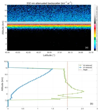
measure-ments of bright, opaque clouds. Low SNR may lead both to missed detections by the surface detection scheme and, within the layer detection algorithm, to missed detections of weaker backscatter signals near the top and apparent base of the opaque layer. The former problem causes the layer two-way transmittance to be set incorrectly to zero and the latter causes the calculated layer integrated attenuated backscatter to be too small. Both of these errors lead to an overestimate of the initial lidar ratio. In such cases the retrieved extinction profile and optical depth will likewise both be overestimated. In Fig. 2, we use simulated data to demonstrate the effect of the different V3 and V4 algorithms on the retrieved ex-tinction profiles. The top of the simulated cloud layer is at 10 km while the base is at 4 km, although it can be seen in Fig. 2a that the signal is totally attenuated at an altitude of about 7.5 km. The V3 retrieval (Fig. 2b), using a fixed lidar ratio of 25 sr and multiple scattering factor of 0.6, can be seen to trend quickly to zero, significantly underestimating the ex-tinction coefficients at all altitudes. In contrast, the V4 re-trieval, which obtains its lidar ratio from the data, stays much closer to the target, trending slightly too low from cloud top to∼8.8 km, then somewhat too high to around 8 km, after which the solution oscillates between being too high and too low. These excursions from the target result from a combina-tion of small differences in the estimated lidar ratio from the target value and from the effects of noise on the signal.
2.2.4 Revised algorithms for adjusting lidar ratios to achieve a successful solution
There are four main potential errors in the inputs supplied to the extinction algorithm. Two of these errors cause the re-trieved particulate extinction to be too high, or cause there to be no possible solution at all. The other two cause the extinc-tion to be too low, or even negative.
If the initial lidar ratio estimate is too high, or the correc-tion for the attenuacorrec-tion caused by overlying layers is too large (i.e., when the optical depths of overlying layers are overes-timated), then the extinction retrieved in the lower layers will be too high, or, in the worst case, not retrievable at all. While retrieval problems in the topmost layers in the atmosphere can usually be attributed to errors in the initial lidar ratios for these layers, as the retrieval process progresses to lower layers that have an increasing number of overlying layers, the retrieval problems are increasingly likely to be at least partially the result of attenuation correction errors. As there is no completely reliable way of determining which of these error sources causes an unsuccessful retrieval, unsuccessful retrievals are addressed by reducing the lidar ratio in both cases. Sometimes the lidar ratio needs to be reduced to val-ues that are far below what is considered to be a valid range. These cases are considered to be failed retrievals and are ter-minated with the QC flag being set to indicate the problem. Where V4 retrievals are terminated at an altitude above the detected base of the feature, a fill value of−333 is inserted in
the retrieval arrays of particulate backscatter and extinction, and their uncertainties, for this altitude and all lower altitudes down to the detected layer base.
When a successful retrieval could not be achieved using a given lidar ratio, the V3 extinction algorithm reduced the lidar ratio by repeatedly applying fixed fractional reductions, initially in steps of 1 % then in steps of 5 %, until either a complete solution was derived or some error condition (e.g., too many solution attempts) occurred [YV09]. The V4 algo-rithm takes a more nuanced approach. V4 adjustments to the lidar ratio in opaque layers are inversely proportional to the average extinction coefficient retrieved over the path from the top of the layer to the point where the retrieval fails with the current lidar ratio, multiplied by both the retrieved two-way particulate transmittance over the same range and an empiri-cally derived scaling constant. This produces smaller adjust-ments where the extinction is higher, as is required to avoid overcorrections. Lidar ratio reductions in opaque layers are limited to a maximum of 1 % on each adjustment. For semi-transparent layers, the fractional reduction is 10 % of the rel-ative uncertainty in the initial lidar ratio.
The opposite problem of the retrieved extinction being too small (or even negative) can occur if the initial lidar ratio is too small or the estimated attenuation for overlying layers is too low. As shown in Y1316, when the optical depth of the layer being analyzed is high, these underestimates can in-troduce significant errors in the extinction retrieval (e.g., as shown in Fig. 2b). However, whereas cases for which the li-dar ratio or the overhead attenuation correction is too large are readily identified because the extinction solution will di-verge before reaching the bottom of a layer, we know of no reliable metric that can unambiguously identify those in-stances where the lidar ratio or the overhead attenuation cor-rection is too low. Consequently, unlike the V3 algorithm, the V4 retrieval does not increase the lidar ratio when negative particulate backscatter coefficients are repeatedly retrieved from positive attenuated backscatter inputs.
As in V3, retrieval uncertainties and retrieval errors in overlying layers propagate into and are amplified by extinc-tion retrievals in underlying layers. While the uncertainties reported in the V4 data products correctly account for the effects of estimated random errors in overlying layers, no es-timates are provided for possible bias errors that might also be incurred. However, the combined random uncertainty in the optical depths of overlying layers can be used to estimate the bias error introduced by the accumulated attenuation cor-rections. Estimates of the total bias error in the lower layer can then be obtained using the various equations and figures in Y1316.
2.2.5 Modification of lidar ratio uncertainties
Figure 2.A comparison of the extinction profiles retrieved by the V4 and V3 algorithms in a simulated totally attenuating ice cloud. The simulated layer has its top at 10 km and its base at 4 km, with a constant extinction coefficient of 2 km−1, yielding an optical depth of 12. The cloud lidar ratio and multiple scattering factor are also uniformly constant values of 33.5 sr and 0.52, respectively. Panel(a)shows a height vs. latitude image of the simulated 532 nm attenuated backscatter coefficients. Panel(b)shows the mean extinction coefficients, averaged across the full horizontal extent of the layer, retrieved by the V3 scheme and the V4 scheme. For both versions, individual extinction profiles were retrieved at 5 km intervals prior to averaging.
by the various lidar ratio determination schemes (i.e., as in Table 1). However, there are some circumstances where the initial lidar ratio uncertainty is modified, or even recalculated completely, within the V4 extinction retrieval algorithm. This final value, whether modified or not, is reported in the V4 data products as the final lidar ratio uncertainty and is ex-pressed as an absolute uncertainty in steradians.
Lidar ratio uncertainties are calculated in constrained re-trievals from the uncertainties in the measured apparent two-way particulate transmittance of the layer under analysis and the integrated particulate attenuated backscatter of the layer, as in Vaughan et al. (2005). In V4, this uncertainty may be reduced if the transmittance plus or minus its uncertainty ex-ceeds the range [0, 1] or if the calculated lidar ratio plus or
so as to maintain the relative uncertainty that is calculated ei-ther from the default values or from the modified values just described.
The rules described above do not apply for lidar ratio un-certainties for opaque water clouds because of lidar “pulse stretching”. Pulse stretching is caused by the broad forward peak of the scattering phase function of the small spherical droplets typically found in water clouds. The broad forward peak causes an increase in off-axis scattering in water clouds. With the increased multiple scattering found at high optical depths (e.g., in opaque water clouds), this off-axis scattering quickly dominates the backscattered signal with increasing penetration into the layer. As lidar range information is mea-sured by the time delay of the backscattered signal, off-axis scattering causes errors in the measured delay, and thereby causes errors in cloud penetration depth measurements. Ow-ing to this loss of range information, the particulate backscat-ter and extinction uncertainties reported for opaque wabackscat-ter clouds in the CALIOP V4 data products are now assigned a fill value of −29, indicating zero confidence in the rela-tionship of the retrieved variables to the related altitude ar-ray. However, we choose to continue to report the retrieved backscatter and extinction for data users who may find value in these quantities as a function of time.
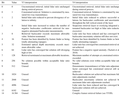
2.2.6 Changes in the extinction quality control (QC) flags
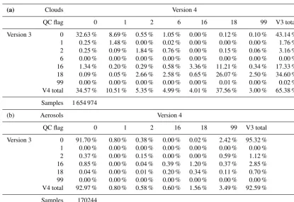
In order to accommodate the modifications described above, and other changes to the algorithms, the extinction QC flags have been modified in V4. The new values and their explana-tions are shown in Table 2. The relative occurrence of each of the QC bits for both clouds and aerosols is provided in Table 3. It can be seen that while nearly 93 % of the aerosol layers have identical QC flags in V3 and V4, identical QC values are found in only 65 % of cloud layers. This difference results mainly from the much higher occurrence of QC=0 in retrievals in aerosol layers.
3 Results of changes
We now present the results of the changes described in Sect. 2, beginning with a study of extinction retrievals in tropical clouds in Sect. 3.1. In Sect. 3.2 we present an anal-ysis of lidar ratios retrieved in ice and water clouds using the new opaque layer algorithm (discussed in Sect. 2.2.3). Sect. 3.3.1 compares the optical depths, retrieved using these lidar ratios with the V3 values obtained using fixed values of the multiple scattering factors and initial lidar ratios. Opti-cal depths retrieved in semi-transparent ice clouds using the V4 and V3 algorithms are compared in Sect. 3.3.2, where we demonstrate the superiority of the V4 results by compar-ing with MODIS C6 data. In Sect. 3.4 we compare V4 and V3 profiles of median extinction coefficient as a function of
temperature and extinction QC. We end with comments and advice on the use of extinction QC values for filtering of data in Sect. 3.5 and provide some caveats on using V4 data in Sect. 3.6.
3.1 Example: retrievals in tropical clouds
In Figs. 3, 4, and 5, we compare the V3 and V4 532 nm analyses of a complex cloud system composed of opaque ice and deep convective clouds observed over Panama and the adjacent seas by CALIOP on 24 April 2010 around 07:18 UTC. The example highlights the impact of the new opaque-layer extinction retrieval algorithm. Figure 3 concentrates on the retrieved backscatter and extinction coefficients, whereas Fig. 4 is mainly concerned with the uncertainties. The level 1 data were extracted from the files CAL_LID_L1-Standard-V4-10.2010-04-24T07-04-53ZN.hdf and CAL_LID_L1-ValStage1-V3-01.2010-04-24T07-04-53ZN.hdf. The level 2 data were extracted from the 5-km cloud profile files CAL_LID_L2_05kmCPro-Standard-V4-10.2010-04-24T07-04-53ZN.hdf and CAL_LID_L2_05kmCPro-Prov-V3-01.2010-04-24T07-04-53ZN.hdf, and the corresponding vertical feature mask files CAL_LID_L2_VFM-Standard-V4-10.2010-04-24T07-04-53ZN.hdf and CAL_LID_L2_VFM-ValStage1-V3-01.2010-04-24T07-04-53ZN.hdf.
Table 2.Extinction quality control flags used in version 3 and version 4.
Bit Value V3 interpretation V4 interpretation
0 0 Unconstrained retrieval; initial lidar ratio unchanged during retrieval process.
Unconstrained retrieval; initial lidar ratio unchanged during retrieval process.
0 1 Constrained retrieval. Solution is constrained by mea-sured two-way transmittance.
Constrained retrieval. Solution is constrained by mea-sured two-way transmittance.
1 2 Initial lidar ratio reduced to prevent divergence of so-lution to infinity.
Initial lidar ratio reduced to achieve successful so-lutions for backscatter coefficients and uncertainties throughout the full vertical extent of the layer 2 4 Initial lidar ratio increased to reduce the number of
negative backscatter coefficients retrieved for non-negative attenuated backscatter measurements.
Suspicious retrieval (layer or overlying integrated at-tenuated backscatter too high or lidar ratio reduction excessive)
3 8 Retrieved backscatter exceeds maximum allowable value. Solution terminated.
Lidar ratio has been reduced and has converged but backscatter uncertainty solution still does not exist. 4 16 Feature has been identified by feature finder as being
totally attenuating (opaque).
Feature has been identified by feature finder as being totally attenuating (opaque).
5 32 Estimated optical depth uncertainty exceeds maxi-mum allowable value.
Lidar ratio has converged but constrained retrieval still not achieved.
6 64 Lidar ratio has converged but solution still diverging high or low.
Feature has a negative signal anomaly. (Tackett et al., 2018)
7 128 Retrieval terminated at maximum allowable iterations. Maximum number of attempts at constrained retrieval exceeded.
8 256 No solution possible within acceptable lidar ratio bounds.
No valid solutions exist within acceptable lidar ratio bounds.
9 512 Unused Denominator (transmittance) of lidar ratio adjustment
factor converged but constrained retrieval still not achieved.
10 1024 Unused Backscatter solution not achieved but maximum lidar
ratio adjustments reached.
11 2048 Unused Backscatter uncertainty solution not achieved but
maximum lidar ratio adjustments reached.
12 4096 Unused Lidar ratio has been reduced and has converged but
backscatter solution still not achieved.
13 8192 Unused Unused
14 16 384 Unused Complex feature retrieval failure (see YV09).
15 32 768 Fill value or no solution attempted. Fill value or no solution attempted.
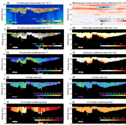
(molecular plus particulate) to give the particulate backscat-ter, the changes in molecular number density result directly in changes to the retrieved profiles of particulate backscat-ter and extinction. Note that the changes to the ozone den-sity profiles (not shown) can also cause differences in the retrieved products, though these are typically quite small.
The retrieved particulate backscatter (To-tal_Backscatter_Coefficient_532) and extinction coefficients (Extinction_Coefficient_532) are plotted in Fig. 3c and e, respectively. Note that, in these products, “Total” refers to the sum of both polarization components of the particulate backscatter, not to the sum of the particulate and molecular components. Figure 3d and f show, respectively, the ratios (V4 divided by V3) of particulate backscatter and extinction coefficients. The differences in the retrieved quantities result not only from the different calibration (Fig. 5a and b) and different molecular density data, but also from the different lidar ratios, plotted in Fig. 3g and h, and multiple
Table 3.A comparison of the V4 and V3 extinction QC flag values for identical layers detected during the years 2007–2010. All QC flag values not shown separately are grouped under QC=99 and indicate the proportion of unsuccessful retrievals:(a)clouds,(b)aerosols.
(a) Clouds Version 4
QC flag 0 1 2 6 16 18 99 V3 total
Version 3 0 32.63 % 8.69 % 0.55 % 1.05 % 0.00 % 0.12 % 0.10 % 43.14 % 1 0.25 % 1.48 % 0.00 % 0.02 % 0.00 % 0.00 % 0.00 % 1.76 % 2 0.25 % 0.09 % 1.84 % 0.76 % 0.00 % 0.15 % 0.06 % 3.16 % 6 0.00 % 0.00 % 0.00 % 0.00 % 0.00 % 0.00 % 0.00 % 0.00 % 16 1.34 % 0.20 % 0.29 % 0.58 % 3.36 % 11.21 % 0.34 % 17.33 % 18 0.09 % 0.05 % 2.66 % 2.58 % 0.65 % 26.07 % 2.50 % 34.60 % 99 0.00 % 0.00 % 0.00 % 0.00 % 0.00 % 0.01 % 0.00 % 0.02 % V4 total 34.57 % 10.51 % 5.35 % 4.99 % 4.01 % 37.56 % 3.00 % 65.38 %
Samples 1 654 974
(b) Aerosols Version 4
QC flag 0 1 2 16 18 99 V3 total
Version 3 0 91.70 % 0.80 % 0.38 % 0.00 % 0.02 % 2.42 % 95.32 % 1 0.00 % 0.00 % 0.00 % 0.00 % 0.00 % 0.00 % 0.00 % 2 0.37 % 0.00 % 0.15 % 0.00 % 0.00 % 0.59 % 1.12 % 16 0.85 % 0.00 % 0.04 % 0.39 % 1.20 % 0.37 % 2.85 % 18 0.04 % 0.00 % 0.01 % 0.20 % 0.34 % 0.11 % 0.70 % 99 0.00 % 0.00 % 0.00 % 0.00 % 0.00 % 0.00 % 0.00 % V4 total 92.97 % 0.80 % 0.58 % 0.60 % 1.56 % 3.49 % 92.59 %
Samples 170244
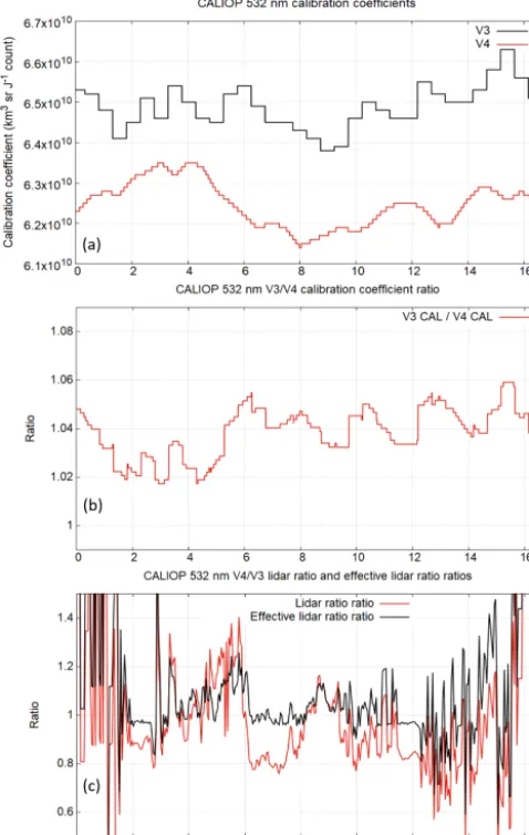
Between the latitudes of∼3 and∼10◦N, where the upper cloud deck is almost continuously opaque, the V4-to-V3 ra-tios of backscatter (Fig. 3d) and extinction (Fig. 3f) increase markedly with penetration depth into the cloud and reach fac-tors of 10 or more near the apparent bases of the cloud. This increase with range results from a combination of the smaller V4 calibration coefficient (Fig. 5a and b), a difference that exceeds 4 % between∼5 and∼9◦N, and the higher V4 ef-fective lidar ratios (Fig. 5c), especially in the latitude ranges
∼4 to∼6◦N and∼8 to∼10◦N, where the lidar ratio dif-ferences are in the range +5 % to +20 % and the increase in backscatter and extinction with range is especially notice-able. Figure 2b gives some insight into how best to inter-pret these large differences. The V4 effective lidar ratios are higher than the V3 values in the latitude ranges 3 to 6 and 8 to 10◦N, and, by scaling the particulate backscatter, lead directly to higher V4 extinctions in these regions. Between 6 and 8◦N, the V4 actual lidar ratios are considerably lower than in V3 and this leads directly to V4 extinctions at the tops of the cloud that are slightly lower than the V3 values, as indicated by the presence of pale blue and grey colors in that region in Fig. 3f. These lower V4 lidar ratios result from the higher V4 multiple scattering values associated with the lower temperatures (Fig. 1a) at the higher cloud attenuated backscatter centroid altitudes in this latitude range. However, note that the effective lidar ratios in this region remain essen-tially identical between V3 and V4 (Fig. 5c).
The implementation of the opaque layer algorithm in V4 results in generally higher effective lidar ratios between the latitudes 3 and 10◦N. Because the retrieval is highly sensi-tive to the initial value of the lidar ratio at such high opti-cal depths, these higher V4 lidar ratios need to be reduced more often than in V3, as indicated by the more frequent oc-currence of QC=18 (dark orange) values in Fig. 4c than in Fig. 4d. However, as mentioned earlier, while the lidar ratios may have been reduced sufficiently to produce successful re-trievals, the final lidar ratios may have still been slightly too large, resulting in retrieved backscatters and extinctions that trend increasingly larger with penetration depth and leading to the high values (dark orange and red regions) near the ap-parent bases of the clouds in Fig. 3d and f. Nevertheless, as shown with simulated data in Fig. 2, the V4 retrievals are substantially more accurate than the V3 retrievals in these opaque regions because the effective lidar ratios were cal-culated from the data as described in Sect. 2.2.3 rather than using a fixed initial value. The higher V4 optical depths re-trieved in the opaque regions of the cloud can be seen in Fig. 4i.
uncertain-Figure 3.A comparison of CALIOP V4 and V3 532 nm analyses of dense clouds observed over Central America and surrounding seas around 07:18 UTC on 24 April 2010. See text for details.
ties in the molecular atmosphere model.) V4 calibration un-certainties are documented in Kar et al. (2018); Getzewich et al. (2018); and Vaughan et al. (2018a). Lidar ratio uncertain-ties are discussed earlier in Sect. 2.1.2 and 2.2.5, and in Kim et al. (2018). As a consequence of these various increases and decreases in relative uncertainties in V4, and the non-linear nature of the lidar equation at high optical depths, there is no simple relationship between the retrieved backscatter and ex-tinction uncertainties in the two data versions. For example, even though the lidar ratio uncertainties have been reduced, the generally higher V4 lidar ratios lead to higher retrieved backscatter and extinction, particularly with increased pene-tration depth, and these result in higher relative uncertainties. Focusing on the main ice cloud layer in Fig. 4e, f, g, and h, in regions where the cloud is not opaque, the V4
uncertain-ties are often lower than the V3 values at the top of the cloud but commonly reach or exceed the V3 values at the base of the cloud. In the region where the cloud is opaque (latitudes
∼3.5 to∼9.5◦N); however, the uncertainties are noticeably lower in V4.
The uncertainties in Fig. 4f and h contribute to the uncer-tainties in the retrieved cloud optical depths shown in Fig. 4j. These cause higher V4 uncertainties between the latitudes
Figure 4.A comparison of CALIOP V4 and V3 532 nm analyses of dense clouds observed over Central America and surrounding seas around 07:18 UTC on 24 April 2010. See text for details.
3.2 Opaque cloud lidar ratios 3.2.1 Ice clouds
The new opaque layer analysis permits the retrieval of the particulate lidar ratio, a parameter of considerable interest. The accuracy of the lidar ratio depends on the accuracy of the integrated attenuated particulate backscatter of the layer and of the determination of its opacity. The accuracy of the first depends on accurate calibration, accurate determination of the existence of overlying layers and correction for their attenuation, and accurate determination of the full vertical extent of the layer down to the altitude at which the backscat-ter signal is extinguished (i.e., where the particulate transmit-tance is truly zero). The accuracy of the second depends on
Figure 5.A comparison of CALIOP V4 and V3 532 nm calibration coefficients and lidar ratios around 07:18 UTC on 24 April 2010. (a)V3 and V4 532 nm calibration coefficients,(b)the ratio of V3 to V4 calibration, and(c)the ratios of the V4 to V3 lidar ratios and effective lidar ratios.
attenuated, the day and night median integrated attenuated backscatters differ by only 3.3 %. In V3, the initial lidar ratio was 25 sr and the multiple scattering factor was 0.6, which (using Eq. 1) corresponds to a layer integrated attenuated backscatter of 0.033 sr−1. The median measured values of the V4 integrated attenuated backscatters differ from this value by∼6 % (daytime) to∼10 % (nighttime). However, as seen in Fig. 6c, the V4 lidar ratios retrieved from these opaque layers are considerably larger than the V3 initial lidar ratio, at 31.5±8.1 sr during the daytime and 31.8±6.7 sr at night. (Recall that the final lidar ratios in V3 were never larger than the initial lidar ratio of 25 sr.)
To demonstrate that the new algorithm is indeed produc-ing lidar ratios that are closer to what is expected in opaque clouds than found for V3 retrievals in Sect. 2.2.3, we repeated
Figure 6.Histograms of(a)cloud geometric extent,(b)532 nm in-tegrated attenuated backscatter, and(c)532 nm lidar ratio for V4 opaque clouds composed of randomly oriented ice (ROI) particles measured during the period 2012–2015. Data are for the top layer in the column only. Statistics are median±median absolute deviation.
4.8 % of the value expected for total attenuation for daytime retrievals and 1.8 % for the nighttime retrievals. The corre-sponding V3 values were 4.4 % and 2.9 %. It can be seen that the major improvement is achieved in the QC=16 re-trievals where the V3 lidar ratios were markedly too low and would have produced retrieved extinction profiles that were also too low (Fig. 2). This improvement results from the bet-ter selection of the initial lidar ratio in V4. A less marked improvement has been achieved in the QC=18 retrievals. This is because the initial V3 lidar ratio was too high, rather than too low, and was subsequently reduced sufficiently to achieve a solution. The marked improvement in V4 is found in the nighttime retrievals. In the January 2010 sample ana-lyzed, QC=18 retrievals occurred more than twice as often in the analysis of nighttime data than in the daytime data. This improvement results mainly from the more finely tuned lidar ratio reduction scheme employed in V4.
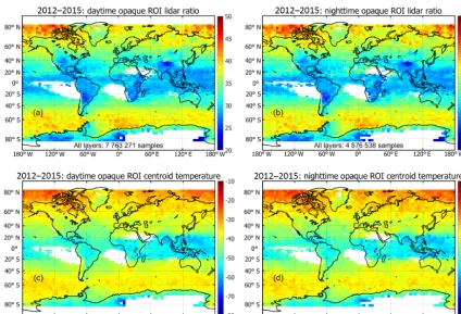
In Fig. 7 we present maps of the global variations in 532 nm lidar ratios for opaque ROI clouds measured during daytime (Fig. 7a) and nighttime (Fig. 7b) during the years 2012 to 2015. The data are for the same clouds as used to create the histograms in Fig. 6. Given the large differences in daytime and nighttime calibrations, the excellent agree-ment shown between the distributions of daytime and night-time lidar ratios is remarkable and gives confidence both in the calibrations and in the new opaque-layer algorithm. The agreement also suggests that the lidar ratio and, by implica-tion, the microphysics in the uppermost regions of opaque ice clouds, do not change significantly between day and night.
A considerable latitudinal variation can be seen in the lidar ratios with the lowest values found over the tropical region and over Antarctica. If the temperature dependence of the li-dar ratio for opaque ROI clouds is the same as that for semi-transparent clouds, this behavior could, at least in part, be ex-plained by the variation in lidar ratio with temperature shown in Fig. 1b. Indeed, in the tropics and over Antarctica, the ice clouds occur at altitudes where the temperature is the coolest, as shown in Fig. 7c and d. There are also some land–ocean differences, which suggest that there could be geographic in-fluences on the cloud microphysics. A more detailed analy-sis, which is beyond the scope of this present work, would be required to determine the causes of the observed distribution.
3.2.2 Water clouds
The new opaque layer algorithms described in Sect. 2.2.3 have also been used to determine the lidar ratio for water clouds. Although retrieval of extinction profiles in opaque water clouds is of low-to-no confidence (as indicated by an uncertainty fill value of−29), the lidar ratio determined from these clouds gives an indication of the possible variation of the lidar ratios that should be used in retrievals in semi-transparent water clouds. In Table 4, we present globally av-eraged data for the period 2008 through 2010 on the lidar ratio retrieved for opaque water clouds measured during the
daytime and nighttime, and on the parameters used in its cal-culation. Filters have been applied to the data to minimize the effects of undetected overlying layers, to ensure that the layers are composed only of liquid water droplets and that the layers are sufficiently robust to ensure reliable results.
We note that the mean daytime lidar ratio of 18.5±2.8 sr is very close to the theoretically expected value, while the nighttime mean is somewhat lower at 17.2±2.9 sr. The low bias in the nighttime lidar ratios is thought to result from a combination of the slow transient recovery of the 532 nm de-tectors in response to the extremely strong signals from these dense water clouds (Hunt et al., 2009) and a diurnal vari-ation in the instrument’s polarizvari-ation gain ratio (PGR) that is used to calculate the depolarization ratios. The non-ideal detector response is responsible for the larger magnitudes of the nighttime integrated attenuated backscatter. The diurnally varying PGR yields depolarization ratios are slightly, but per-sistently, lower at night leading to multiple scattering factors that are slightly, but persistently, higher. This combination of high biases in integrated attenuated backscatters and multiple scattering factors at night leads to low biases in the nighttime lidar ratio estimates.
Figure 7.Global distribution of lidar ratios measured in opaque ROI clouds (a)by day and (b)by night between 2012 and 2015. The corresponding cloud 532 nm attenuated backscatter centroid temperatures are shown in panels(c)and(d).
3.3 Cloud optical depths 3.3.1 Opaque clouds
We turn now to the fractional optical depths retrieved in opaque clouds using the new methods. Readers are reminded that the CALIOP optical depths reported for opaque clouds are retrieved only over the range from the top of the cloud down to the altitude at which the signal is totally attenuated (i.e., when the signal is indistinguishable from the ambient noise). Consequently, CALIOP opaque cloud optical depth estimates cannot be compared with cloud optical depths mea-sured by passive instruments. In Fig. 9, we present a com-parison of the V3 and V4 distributions of optical depths for the topmost opaque (QC=16 and QC=18) ROI clouds de-tected during 2012–2015. There are several features of note. Most obvious is the marked difference between the V3 and V4 mean optical depths for these opaque clouds. The V3 dis-tributions for day and night peak at optical depths in the range 1.2 to 1.5, or effective optical depths of 0.72 to 0.9. Such low values are insufficient to cause complete attenuation of the CALIOP signal and reinforce our conclusion that the V3 li-dar ratios, and, consequently, optical depths, are considerably underestimated.
The second notable feature is the large difference in the daytime and nighttime V4 distributions. This difference is
explained by the dramatic shift from QC=16 to QC=18 that occurred in the V4 daytime opaque cloud retrievals. The main nighttime peak at∼6.6 corresponds to retrievals with QC=16. Optical depths smaller than about 6 correspond to the far fewer nighttime retrievals in which the lidar ratio required reduction (QC=18). Conversely, for the daytime data, the small secondary peak at an optical depth of∼6.6 corresponds to relatively few retrievals in which the lidar ra-tio has not been reduced (QC=16), whereas the much larger peak at∼4 corresponds to those retrievals where the lidar ratio has been reduced. The much broader daytime QC=18 peak in V4, when compared with the sharper peaks in V3, re-sults largely from the new lidar ratio reduction scheme with its finer and variable adjustments.
Table 4.Statistical characterization of global measurements of opaque water clouds during 2008–2010, where the clouds were the only layers detected in a 5 km averaged column. The integrated attenuated backscatter, layer-integrated volume depolarization ratio, and layer-integrated attenuated backscatter color ratio are measured over the detected cloud geometrical thicknesses. The multiple scattering factors are derived using the method of Hu et al. (2007), and the lidar ratios are retrieved using Eq. (1). MAD is the median absolute deviation andNis the number of unique cloud layers used in the calculations. Data have been filtered to minimize the effects of potentially undetected overlying layers. Layer integrated attenuated backscatter is limited to the range (0.021–0.111 sr−1), layer depolarization to the range (0.03–0.39), layer attenuated color ratio to the range (0.90–1.50) and overlying attenuated backscatter to values less than 0.02 sr−1, and (for nighttime layers only) greater than zero.
Geometric Integrated Depolarization Attenuated Multiple Lidar thickness attenuated ratio backscatter scattering ratio
(km) backscatter color factor (sr)
(sr−1) ratio
Daytime N=7 298 084
Minimum 0.090 0.021 0.030 0.900 0.193 0.14
Maximum 10.493 0.111 0.390 1.500 0.887 59.74
Median 0.599 0.064 0.211 1.189 0.425 18.27
MAD 0.288 0.011 0.047 0.052 0.084 1.94
Mean 0.747 0.065 0.211 1.189 0.436 18.54
Standard deviation 0.443 0.013 0.058 0.071 0.105 2.76
Nighttime N=3 479 891
Minimum 0.090 0.021 0.030 0.900 0.193 0.13
Maximum 12.350 0.111 0.390 1.500 0.887 51.70
Median 0.928 0.067 0.203 1.167 0.438 16.89
MAD 0.427 0.012 0.046 0.045 0.085 1.72
Mean 1.152 0.068 0.204 1.165 0.448 17.26
Standard deviation 0.730 0.015 0.056 0.061 0.105 2.86
2009 for a detailed explanation.) These artifacts are not seen in V4 thanks to the refined reduction of the lidar ratios de-scribed in Sect. 2.2.4.
3.3.2 Semi-transparent clouds
Global maps of the nighttime optical depths for semi-transparent high confidence ROI clouds (QC=0, 1 or 2) are presented in Fig. 10. For both V3 (Fig. 10a) and V4 (Fig. 10b), the optical depths in the tropical regions, partic-ularly over the oceans, are considerably lower than at higher latitudes. The V4/V3 COD ratios (Fig. 10c) are higher at middle to high latitudes and suggest that the changes between V4 and V3 differ, to some extent, over land and ocean. For example, the lower V4/V3 ratios over South America, Cen-tral and Southern Africa, and especially over the Himalayas are rather distinct. In general, the area-weighted average opti-cal depths are considerably higher for V4 (0.266) than for V3 (0.137). The dominant cause of the larger V4 optical depths is the higher lidar ratios (Fig. 1b) used in the V4 retrievals.
As mentioned previously, Holz et al. (2016) showed that while CALIOP V3 constrained (QC=1) optical depths in semi-transparent ice clouds agreed rather well with MODIS C6 optical depths, the unconstrained retrievals (QC=0, 2) were substantially smaller than the MODIS values. As a conclusive demonstration of the major improvement in the V4 optical depths, in Fig. 11 we compare MODIS C6
Figure 8.Mean global distribution of daytime opaque water clouds during 2008–2010;(a)532 nm lidar ratios,(b)sample counts. Data have been filtered as described in the caption for Table 4.
Figure 9.Distributions of the apparent optical depths measured in opaque ROI clouds during 2012–2015 and processed using the V3 and V4 algorithms.
to show a rather different height and temperature dependence from that shown by the V3 retrievals. We examine these dif-ferences in this section.
In Fig. 12, we compare V3 and V4 cloud extinction coef-ficients plotted as a function of temperature. The profiles are
Figure 10. Median cloud optical depths (CODs) for semi-transparent, high-confidence nighttime ROI clouds for the pe-riod March to May 2010 inclusive, nighttime only. The area-weighted average optical depths from the maps are 0.137 for V3 (77 230 457 samples) and 0.266 for V4 (78 808 302 samples).
Figure 11.A comparison of collocated MODIS C6 optical depths with CALIOP optical depths retrieved using the V3 (a, c) and V4(b, d)algorithms for January 2008(a, b)and July 2008(c, d). Data were sampled over oceans in daytime and from both hemi-spheres between 30 and 60◦ latitude. Color scale indicates num-ber of samples (on log 10 scale) normalized to the maximum value in each panel. The 1 km MODIS C6 samples were collocated with the center of the CALIOP 5 km samples. Data were obtained from the ICARE CALTRACK product. Samples were restricted to cases where there was only one V4 cloud in the column with no bound-ary layer clouds cleared at single shot resolution. All V4 clouds were identified as high confidence ROI, whereas the V3 phase was ice (either ROI or HOI) and the MODIS phase was ice. V4 data were restricted to QC=0 or QC=1, but all transparent ice clouds were accepted in V3. Samples were further restricted to cases where cloud tops and bases were identical in V4 and V3.
For unconstrained retrievals, in which the lidar ratio is unchanged from the initial value (QC=0, Fig. 12a, b), the median extinction profiles in V4 are larger at all tempera-tures above −72◦C and this difference increases with tem-perature and as would be expected from Fig. 1b, where the V4 lidar ratios are shown to increase relative to the V3 val-ues. There are also fewer QC=0 retrievals in V4 than in V3 (Fig. 12a), mostly because many retrievals that were as-signed QC=0 in V3 are accepted as constrained retrievals in V4 (see Sect. 2.2.1), so that clouds of small optical depth that were QC=0 in V3 are QC=1 in V4. The smaller oc-currence of QC=0 retrievals in V4 and the increase in re-trievals with QC=1 can be seen in Fig. 12a and c, respec-tively. A closer agreement between daytime and nighttime QC=0 extinction profiles is seen in V4.
The large increase in the number of constrained retrievals (QC=1) in V4 occurs for all temperature levels for both nighttime and, particularly, daytime retrievals (Fig. 12c). The
increase in nighttime retrievals is greater at higher altitudes (i.e., lower temperatures) than for the daytime retrievals, pos-sibly because the SNR at the higher altitudes is often too low by day to permit detection of tenuous features or reli-able measurement of their effective transmittances. The V4 median extinction coefficients are lower than the V3 values at temperatures below ∼ −20◦C. This is explained by the larger fraction of clouds of small optical depths in the pop-ulation of QC=1 retrievals in V4 than in V3. The mean optical depth for QC=1 retrievals in V4 is 0.560±0.599, whereas for V3 the QC=1 mean is 0.988±0.558. This dif-ference is the direct result of the algorithm changes described in Sect. 2.2.1.
The use of higher lidar ratios in V4 would be expected to lead to a greater number of retrievals in which the lidar ra-tio needs to be reduced in semi-transparent clouds (QC=2, Fig. 12e). While this is seen in the nighttime comparisons, the daytime comparison is not as straightforward. Given the use of generally higher ice cloud lidar ratios in V4 than in V3, the almost uniformly lower V4 extinction coefficients in V4 than in V3 for QC=2 (Fig. 12f) is, at first, surprising. However, in V4, as explained in Sect. 2.2.2, the lidar ratio is reduced if the calculation of either the backscatter or its uncertainty fails. In V3 it was not reduced if the uncertainty calculation failed and the uncertainty was simply limited to 99.99 units. The consequence is that the final, reduced, lidar ratios in V4 are lower than in V3 and this results in lower extinction coefficients. It is important, too, to remember that QC=2 is a very special case. In V4, layers that are origi-nally assigned QC=2 get additional scrutiny and, if the so-lutions are found to be unrealistic, bit 2 of the QC flag is set, so that instead of being assigned QC=2 they are now as-signed QC=6. This additional quality assurance test, which was not implemented in V3, helps to further explain why the V3 extinction coefficients are larger than the V4 values for QC=2. This is yet another case of not having the same un-derlying cloud populations, even though the QC values are the same. Note, in particular, the huge decrease in the num-ber of daytime V4 retrievals at higher temperatures, which occur at the lower part of the cloud layer (Fig. 12e), and may be a result, in part, of changes to the ice–water phase algo-rithm (Avery et al., 2018). In V4, some of the erroneous so-lutions that were left intact in the V3 analyses have now been identified and labeled with the correct QC flag.
diurnal variations in the calibration coefficients, gives confi-dence in the new algorithm and also in the general perfor-mance of the new surface detection algorithm, which deter-mines layer opacity. The marked reduction in the number of daytime QC=16 (Fig. 12g) retrievals and corresponding in-crease in QC=18 (Fig. 12i) retrievals result both from these factors and from the general increased likelihood of failures in the initial retrievals when using higher lidar ratios, partic-ularly at high optical depths. While there has been a∼60 % reduction in the total (day plus night) QC=16 retrievals in V4, there has been a∼100 % increase in the total number of QC=18 retrievals. The total number of successful opaque layer retrievals has increased by only∼6 %.
Finally, a comment must be made about the kink, or in-crease in slope, in almost all of the V3 and V4 extinction profiles at a temperature of∼ −15◦C. It is possible that this results from a change in phase near the bases of clouds. Cur-rently, the same ice water phase is assigned to all levels of a detected layer. A retrieval in a layer determined to be ROI would be assigned an initial lidar ratio, which would be con-siderably larger than that for a water cloud, for the whole depth of the layer. While this would produce a satisfactory result in the regions where the particles were truly ROI, in regions where the particles were water droplets or a mixture of water and ice, the ROI lidar ratio would be too large and an overestimation the extinction coefficient would result.
3.5 Comments and advice on the use of CALIOP extinction QC values
Extinction QC flags are often used to filter data for quality during analyses, and the question is sometimes asked as to which values indicate retrievals that are “trustworthy” or “re-liable”. Unfortunately, there is no absolute or straightforward answer to this question and the QC flags should be used while bearing in mind various caveats. That said, only those data with QC flag values of 0, 1, 2, 16, and 18 should be used for reliable scientific analyses.
Constrained retrievals (QC=1) are generally regarded as the highest quality retrievals. However, even QC=1 re-trievals will sometimes be affected by calibration errors or errors caused by missed detection or incorrect calculation of the attenuation of overlying layers. These situations are con-sidered as normalization errors and their effects described in Y1316. Constrained retrievals for which the final lidar ra-tio approaches the specified limits (0.05 to 250 sr) should be considered suspicious, as they most likely represent a mis-match (due to noise) between the measurements of integrated attenuated backscatter and apparent two-way transmittance for a given layer. The highest quality constrained retrievals are found in those features that (a) are the topmost layer de-tected, (b) have relatively low values of both the measured two-way transmittance and its relative uncertainty, and (c) have low values of overlying attenuated backscatter.
Con-Figure 12.A comparison of version 4.1 and version 3.3 median ROI cloud extinction profiles measured during September 2014. All clouds were the topmost detected features in the atmospheric column. Daytime and nighttime median extinctions are plotted as functions of temperature and QC value in the column on the right while the corresponding numbers of contributing samples are plot-ted in the column on the left.
strained retrievals account for∼11 % of all V4 cloud solu-tions and∼1 % of all aerosol solutions.
Unconstrained retrievals in semi-transparent layers in which the lidar ratio has not been reduced (QC=0) usually occur in layers of low particulate extinction and low optical depth. The higher the optical depth, the higher the sensitiv-ity on the lidar ratio (Y1316). Because the optical depths are low, so too are the internal two-way transmittance correc-tions. The result is that the retrieved particulate backscatter profiles are relatively insensitive to errors in the lidar ratio and thus are of good quality in low optical depth layers. How-ever, the retrieved particulate extinction profile, because it is obtained by multiplication of the retrieved backscatter profile by the lidar ratio, will reflect any errors that exist in the lidar ratio. Unconstrained retrievals account for∼41 % of all V4 cloud solutions and∼92 % of all aerosol solutions.