Novel automated inversion algorithm for temperature reconstruction using gas isotopes from ice cores

https://doi.org/10.5194/cp-14-763-2018

© Author(s) 2018. This work is distributed under the Creative Commons Attribution 4.0 License.

Novel automated inversion algorithm for temperature

reconstruction using gas isotopes from ice cores

Michael Döring1,2and Markus C. Leuenberger1,2

1_{Climate and Environmental Physics, University of Bern, Bern, Switzerland} 2_{Oeschger Centre for Climate Change Research (OCCR), Bern, Switzerland}

Correspondence:Michael Döring ([email protected])

Received: 3 July 2017 – Discussion started: 17 July 2017

Revised: 30 April 2018 – Accepted: 12 May 2018 – Published: 12 June 2018

Abstract. Greenland past temperature history can be

re-constructed by forcing the output of a firn-densification and heat-diffusion model to fit multiple gas-isotope data (δ15N or

δ40Ar orδ15Nexcess) extracted from ancient air in Greenland

ice cores using published accumulation-rate (Acc) datasets. We present here a novel methodology to solve this in-verse problem, by designing a fully automated algorithm. To demonstrate the performance of this novel approach, we be-gin by intentionally constructing synthetic temperature histo-ries and associatedδ15N datasets, mimicking real Holocene data that we use as “true values” (targets) to be compared to the output of the algorithm. This allows us to quantify uncertainties originating from the algorithm itself. The pre-sented approach is completely automated and therefore min-imizes the “subjective” impact of manual parameter tuning, leading to reproducible temperature estimates. In contrast to many other ice-core-based temperature reconstruction meth-ods, the presented approach is completely independent from ice-core stable-water isotopes, providing the opportunity to validate water-isotope-based reconstructions or reconstruc-tions where water isotopes are used together with δ15N or

δ40Ar. We solve the inverse problem T(δ15N, Acc) by us-ing a combination of a Monte Carlo based iterative approach and the analysis of remaining mismatches between modelled and target data, based on cubic-spline filtering of random numbers and the laboratory-determined temperature sensitiv-ity for nitrogen isotopes. Additionally, the presented recon-struction approach was tested by fitting measuredδ40Ar and

δ15Nexcess data, which led as well to a robust agreement

be-tween modelled and measured data. The obtained final mis-matches follow a symmetric standard-distribution function. For the study on synthetic data, 95 % of the mismatches

com-pared to the synthetic target data are in an envelope between 3.0 to 6.3 permeg forδ15N and 0.23 to 0.51 K for temper-ature (2σ, respectively). In addition to Holocene tempera-ture reconstructions, the fitting approach can also be used for glacial temperature reconstructions. This is shown by fitting of the North Greenland Ice Core Project (NGRIP)δ15N data for two Dansgaard–Oeschger events using the presented ap-proach, leading to results comparable to other studies.

1 Introduction

2016) and human societies (Holmgren et al., 2016; Lespez et al., 2016). Precise high-resolution temperature estimates can contribute significantly to the understanding of these mech-anisms. Ice-core proxy data offer multiple paths for recon-structing past climate and temperature variability. The stud-ies of Cuffey et al. (1995), Cuffey and Clow (1997) and Dahl-Jensen et al. (1998) demonstrate the usefulness of invert-ing the measured borehole-temperature profile for surface-temperature-history estimates for the investigated drilling site using a coupled heat- and ice-flow model. Because of smoothing effects due to heat diffusion within an ice sheet, this method is unable to resolve fast temperature oscilla-tions and leads to a rapid reduction of the time resolution towards the past. Another approach to reconstruct past tem-perature is based on the calibration of water-stable isotopes of oxygen and hydrogen (δ18Oice,δDice) from ice-core

water-samples assuming a constant (and mostly linear) relationship between temperature and isotopic composition due to frac-tionation effects during ocean evaporation, cloud formation and snow and ice precipitation (Johnsen et al., 2001; Stuiver et al., 1995). This method provides a rather robust tool for reconstructing past temperature for times where large tem-perature excursions occur when an adequate relationship is used (Dansgaard–Oeschger events, glacial–interglacial tran-sitions; Dansgaard et al., 1982; Johnsen et al., 1992). Also, in the Holocene where Greenland temperature variations are comparatively small, seasonal changes of precipitation as well as of evaporation conditions at the source region may contribute to water-isotope-data variations (Huber et al., 2006; Kindler et al., 2014; Werner et al., 2001). A relatively new method for ice-core-based temperature reconstructions uses the thermal fractionation of stable isotopes of air com-pounds (nitrogen and argon) within a firn layer of an ice sheet (Huber et al., 2006; Kindler et al., 2014; Kobashi et al., 2011; Orsi et al., 2014; Severinghaus et al., 1998, 2001). The mea-sured nitrogen- and argon-isotope records of air enclosed in bubbles in an ice core can be used as a paleothermometer due to (i) the stability of isotopic compositions of nitrogen and ar-gon in the atmosphere at orbital timescales and (ii) the fact that changes are only driven by firn processes (Leuenberger et al., 1999; Mariotti, 1983; Severinghaus et al., 1998). To ro-bustly reconstruct the surface temperature for a given drilling site, the use of firn models describing gas and heat diffusion throughout the ice sheet is necessary to decompose the grav-itational from the thermal-diffusion influence on the isotope signals.

This work addresses two issues relevant for temperature reconstructions based on nitrogen and argon isotopes. First, we introduce a novel, entirely automated approach for invert-ing gas-isotope data to surface-temperature estimates. For that, we force the output of a firn-densification and heat-diffusion model to fit gas-isotope data. This methodology can be used for many different optimization tasks not restricted to ice-core data. As we will show, the approach works in ad-dition toδ15N for all relevant gas-isotope quantities (δ15N,

δ40Ar,δ15Nexcess) and for Holocene and glacial data as well.

Furthermore, the possibility of fitting all relevant gas-isotope quantities, individually or combined, makes it possible, for the first time, to validate the temperature solution gained from a single isotope species by comparison to the solu-tion calculated from other isotope quantities. This approach is a completely new method which enables the automated fitting of gas-isotope data without any manual tuning of pa-rameters, minimizing any potential “subjective” impacts on temperature estimates as well as working hours. Also, ex-cept for the model spin-up, the presented temperature recon-struction approach is completely independent from water-stable isotopes (δ18Oice,δDice), which provides the

oppor-tunity to validate water-isotope-based reconstructions (e.g. Masson-Delmotte, 2005) or reconstructions where water iso-topes are used together withδ15N orδ40Ar (e.g. Capron et al., 2010; Huber et al., 2006; Landais et al., 2004). To our knowledge, there are only two other reconstruction methods independent from water-stable isotopes that have been ap-plied to Holocene gas-isotope data, without a priori assump-tion on the shape of a temperature change. The studies from Kobashi et al. (2008a, 2017) use the second-order parame-terδ15Nexcess to calculate firn-temperature gradients, which

are later temporally integrated from past to future over the time series of interest using the firn-densification and heat-diffusion model from Goujon et al. (2003). Additionally Orsi et al. (2014) use a linearized firn-model approach together withδ15N andδ40Ar data to extract surface-temperature his-tories. The method presented here can be used when noδ40Ar data are available, which is often the case becauseδ40Ar is a more analytically challenging measurement and is not as commonly measured asδ15N and further allows a compari-son among solutions obtained from any of the available iso-tope quantities.

Second, we investigate the accuracy of our novel fitting approach by examining the method on different synthetic nitrogen-isotope and temperature scenarios. The aim of this work is to study the uncertainties emerging from the algo-rithm itself. Furthermore, the focal questions in this study are what the minimal mismatch inδ15N for Holocene-like data we can reach is and what the implication for the final temperature mismatches is. Studying and moreover answer-ing these questions makes it mandatory to create well-defined

δ15N targets and related temperature histories. It is impossi-ble to answer these questions without using synthetic data in a methodology study. The aim is to evaluate the accu-racy and associated uncertainty of the inverse method itself to then later apply this method to realδ15N,δ40Ar orδ15Nexcess

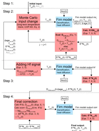
Figure 1.Schematic illustration of the presented gas-isotope fitting algorithm. The algorithm is implemented in four steps: step 1: first-guess input calculation; step 2: iteratively Monte Carlo based input change (indicated by the open half cycles); step 3: signal complementation with high-frequency information; step 4: final correction. In contrast to the synthetic data study on Holocene-like data where the accumulation input Acc(t) was fixed, for the proof of concept on glacial data, the accumulation and temperature input was iteratively changed in parallel indicated by the grey variables Accg,0and Accmc,fin. For the glacial study, only steps 1 and 2 were used.

2 Methods and data

2.1 Reconstruction approach

The problem that we deal with is an inverse problem, since the effect, observed as δ15N variations, is dependent on its drivers, i.e. temperature and accumulation-rate changes. Hence, the temperature that we would like to reconstruct depends on δ15N and accumulation-rate changes. To solve this inverse problem, the firn-densification and heat-diffusion model (from now on referred to as firn model), which is a non-linear transfer function of temperature and accumulation rate to firn states and relates toδ15N values, is run iteratively

to match the modelled and measuredδ15N values (or other gas species). The automated procedure is significantly more efficient and less time consuming than a manual approach. The Holocene temperature reconstruction is implemented by the following four steps (Fig. 1):

– Step 1: a prior temperature input (first guess) is con-structed, which serves as the starting point for the opti-mization.

– Step 2: a long-term solution which passes through the

the smooth solution contains all long-term temperature trends (centuries to millennia) as well as firn-column height changes (temperature and accumulation-rate de-pendent) that drive the gravitational background signal inδ15N.

– Step 3: the long-term temperature solution is comple-mented by superimposing short-term information di-rectly extracted from the δ15N data (here synthetic target data). This step adds short-term temperature changes (decadal) in the same time resolution as the data.

– Step 4: the gained temperature solution is further cor-rected using information extracted from the mismatch between the synthetic target and modelledδ15N time se-ries.

The functionality of the presented inversion algorithm is schematically displayed in Fig. 1. It guides the reader through chapters and documents where variables, listed in Table 1, are in use. In the following, a detailed description of each step is given.

2.1.1 Step 1: prior input

The starting point of the optimization procedure is the first guess. To construct the first-guess temperature inputTg,0(t),

a constant temperature of−29.6◦C is used for the complete Holocene section, which corresponds to the last value of the temperature spin-up (Fig. 2b).

2.1.2 Step 2: Monte Carlo type input generator – generating long-term solutions

During the second step of the optimization, the prior tem-perature inputTg,0(t) from step 1 is iteratively (j) changed

following a Monte Carlo approach. The basic idea of the Monte Carlo approach is to generate smooth temperature in-putsTmc,j(t) by superimposing low-pass-filtered valuesPj of uniformly distributed random valuesPr,j on the prior in-putTmc,j−1. Then, the new input is fed to the firn model and

the mismatch D_δ15_N

mc,j (with X≡δ

15_N

mc,j) between the modelledδ15Nmc,j (hereXmod), calculated from the model

output, and the syntheticδ15Nsyn(hereXtarget) is computed

for every time step (i) of the target dataδ15Nsynaccording to

DX= 1

n

Xn

i=1 DX,i = 1 n Xn

i=1

Xtarget,i−Xmod,i

. (1)

(Note: if not otherwise stated, all mismatches in this study labelled with “D” are calculated similar to Eq. 1.)

D_δ15_N

mc serves as the criterion which is minimized

dur-ing the optimization in step 2. If the mismatchD_δ15_N mc,j de-creases compared to the prior input (Tmc,j−1,Dδ15_N

mc,j−1),

the new input is saved and used as the new guess

(Tg,j=Tmc,j). This procedure is repeated until conver-gence is achieved, leading to the final long-term temperature

Tmc,fin(t). Table 2 lists the number of improvements and

iter-ations performed for the different synthetic datasets. The perturbation of the current guessTg,j is conducted in the following way: letTg,0=Tg,0(t) be the vector

contain-ing the prior temperature input. A second vector (Pr,1) with

the same number of elementsnmcasTg,0is generated,

con-tainingnmcuniformly distributed random numbers within the

limits of an also randomly (equally distributed) chosen stan-dard deviation (SD). SD is chosen from a range of 0.05–0.50, which means that the maximum allowed perturbation of a single temperature valueT(t0) is in a range of±5 to±50 %. Creating the synthetic frequencies,Pr,1is low-pass filtered

using cubic-spline filtering (Enting, 1987) with an equally distributed random cut-off period (COP) in the range of 500 to 2000 years generating the vectorP1. Hereby the low-pass

filtering ofPr,1reduces the amplitudes of the perturbation of

Tg,0. The new surface temperature inputTmc,1is calculated

fromP1according to

Tmc,1=TTg,0·(1ˆ+P1). (2)

The superscript “T” stands for transposed and1 is theˆ nby 1 matrix of ones.

This approach provides a high potential for parallel com-puting. In this study, an eight-core computer was used, gen-erating and running eight different inputs ofTmc

simulta-neously, minimizing the time to find an improved solution. For example, during the 706 iterations for scenario S2, about 5600 different inputs were created and tested, leading to 351 improvements (see Table 2). Since it is possible to find more than one improvement per iteration step due to the par-allelization on eight CPUs, the solution giving the minimal misfitD_δ15_N

mc,j is chosen as new first-guess for the next it-eration step. This leads to a decrease of the used improve-ments for the optimization (e.g. for S2, 172 of the 351 im-provements were used). Additionally, a first gas-age scale (1agemc,fin(t)) is extracted from the model using the last

im-proved conditions, which will then be used in step 3.

2.1.3 Step 3: adding short-term (high-frequency) information

In step 3, the missing short-term temperature history provid-ing a suitable fit between modelled and syntheticδ15N data is directly extracted from the pointwise mismatchD_δ15_N

mc,fin(t),

between the modelledδ15Nmc,fin(t) obtained in step 2 and the

syntheticδ15Nsyntarget. Note that for a real reconstruction,

this mismatch is calculated using the measured δ15Nmeas

dataset instead of the synthetic one.D_δ15_N

mc,fin(t) can be

in-terpreted in first order as the detrended high-frequency signal of the syntheticδ15Nsyntarget.Dδ15_N

mc,fin(t) is transferred to

the gas-age scale using1agemc,fin(t) provided by the

Table 1.Used variables and acronyms with their explanations.

Variable Explanation

αT thermal-diffusion constant calculated from Eq. (12)

α18_O slope forδ18Oicecalibration (surface-temperature spin-up), Eq. (13) Acc accumulation-rate data

Accg,0 first-guess (prior) input accumulation-rate data

Accmc,fin modelled accumulation-rate data from the final Monte Carlo output

β intercept forδ18Oicecalibration (surface-temperature spin-up), Eq. (13) COP cut-off period for cubic-spline filtering

corr index related to the final correction step (step 4) CZ convective zone

D mean mismatch (general) calculated from Eq. (1)

D(t),D_i pointwise mismatches (general)

D_δ15_N mean mismatch ofδ15N

D_δ15_N

corr mean mismatch ofδ

15_{N (δ}15_N

synvs.δ15Ncorr) calculated from the output of the final correction (step 4)

D_δ15_N

g,0 mean mismatch ofδ

15_{N (δ}15_N

synvs.δ15Ng,0) calculated from the output of the first-guess data

D_δ15_N

hf mean mismatch ofδ

15_{N (δ}15_N

synvs.δ15Nhf) calculated from the output of the high-frequency step (step 3)

D_δ15_N

mc,fin mean mismatch ofδ

15_{N (δ}15_N

synvs.δ15Nmc,fin) calculated from the final Monte Carlo output (step 2)

D_gl minimization criterion for the proof of concept on glacial data as used in Eq. (14)

D_T mean mismatch of temperature

D_Tcorr mean mismatch of temperature (Tsynvs.Tcorr) calculated from the output of the final correction (step 4)

D_Tg,0 mean mismatch of temperature calculated fromTsynvs.Tg,0

D_Thf mean mismatch of temperature (Tsynvs.Thf) calculated from the output of the high-frequency step (step 3)

D_Tmc mean mismatch of temperature calculated from the final output of the Monte Carlo step (step 2)

δ15Ncorr modelledδ15N signal from the output of the final correction (step 4)

δ15Ngrav gravitational component of theδ15N signal

δ15Ng,0 modelledδ15N signal from the output of the first-guess data (step 1)

δ15Nhf modelledδ15N signal from the output of the high-frequency step (step 3)

δ15Nmc,fin modelled (smooth)δ15N signal from the final Monte Carlo output (step 2)

δ15Nmod modelledδ15N signal (general)

δ15Ntherm thermal-fractionation/thermal-diffusion component of theδ15N signal

δ15Nsyn syntheticδ15N target (fitting target)

1age gas-age – ice-age difference

1age_mc,fin final gas-age – ice-age output from the Monte Carlo step (step 2)

1δ15Ncv δ15N correction values calculated from1δ15Nmaxand1δ15Nmin

1δ15Nmax δ15N correction values calculated from the linear dependency of xcfmax,δ15_N

1δ15Nmin δ15N correction values calculated from the linear dependency of xcfmin,δ15_N

1m molar mass-difference between the heavy and light isotopes

1T high-frequency temperature signal obtained from Eq. (3) (step 3)

ε_δ15_N uncertainty of theδ15N data as used in Eq. (14)

ε₁age uncertainty of the1age data as used in Eq. (14)

g gravitational acceleration

g,0 index related to the first-guess (prior) data (step 1) hf index related to the high-frequency step (step 3)

i time index

IF “integrated factor” calculated from Eq. (6), needed for the final correction step (step 4)

j running index for the Monte Carlo iterations (step 2)

lagmax time lag attributed to the maximum of the sample cross-correlation function (xcf), (general) lag_max,δ15_N time lag attributed to the maximum of the sample cross-correlation function (xcf) of IF(t) vs.D_δ15_N

hf(t)

lagmax,T time lag attributed to the maximum of the sample cross-correlation function (xcf) of IF(t) vs.DThf(t)

lagmin time lag attributed to the minimum of the sample cross-correlation function (general) lag_min,δ15_N time lag attributed to the minimum of the sample cross-correlation function of IF(t) vs.D_δ15_N

hf(t)

lagmin,T time lag attributed to the minimum of the sample cross-correlation function of IF(t) vs.DThf(t)

mc index related to the Monte Carlo step (step 2) mc,fin index related to the final Monte Carlo output (step 2)

Table 1.Continued.

Variable Explanation

n_mc length of the Holocene temperature vectors (w/o spin-off)

N2,i thermal-diffusion sensitivity calculated from Eq. (4)

P_j spline-filteredP_r,j

P_r,j vector containingnmcuniformly distributed random numbers

R ideal gas constant

ρ_ice ice density

ρ_LID lock-in density, density threshold for calculatingz_LID

SD standard deviation of the random numbers forPr,j

σ_δ15_N

corr standard deviation ofDδ15Ncorr(t) (=Dδ15Ncorr,i) 2σ_δ15_N

corr,95 95 % quantile ofDδ15Ncorr(t) (=Dδ15Ncorr,i)

σ_δ15_N

hf standard deviation ofDδ15Nhf(t) (=Dδ15Nhf,i)

σ_T

corr standard deviation ofDTcorr(t) (=DTcorr,i) 2σ_T

corr,95 95 % quantile ofDTcorr(t) (=DTcorr,i)

σ_T

hf standard deviation ofDThf(t) (=DThf,i)

T,T_firn mean firn temperature

T_bottom temperatures at the bottom of the diffusive firn layer

Tcorr temperature signal calculated from the final correction step (step 4)

T_g,0 first-guess (prior) temperature input

T_hf temperature signal calculated from the high-frequency step (step 3)

T_mc,j Monte Carlo temperature guess for iterationj

T_mc,fin (smooth) temperature modelled from the final Monte Carlo output (step 2)

T_spin surface-temperature spin-up

T_surf temperatures at the top of the diffusive firn layer

wRMSE mean squared errors weighted with data uncertainty as used in Eq. (14) xcf/XCF sample cross-correlation function, needed for the final correction step (step 4) xcfmax maximum of the sample cross-correlation function (general)

xcf_max,δ15_N maximum of the sample cross-correlation function of IF(t) vs.D_δ15_N hf(t)

xcfmax,T maximum of the sample cross-correlation function of IF(t) vs.DThf(t)

xcfmin minimum of the sample cross-correlation function

xcf_min,δ15_N minimum of the sample cross-correlation function of IF(t) vs.D_δ15_N hf(t)

xcfmin,T minimum of the sample cross-correlation function of IF(t) vs.DThf(t)

X_mod modelled data (general), can beδ15N,T or measured data (δ40Ar,δ15Nexc)

X_target fitting target (general), can be syntheticδ15Nsyn,Tsynor measured data (δ40Ar,δ15Nexc)

z_LID, LID lock-in depth

Table 2.Summary for the Monte Carlo approach: mismatchDg,0between the modelledδ15N (or temperature) values using the first-guess input and the syntheticδ15N (or temperature) target for each scenario.Dmcis the mismatch between the modelledδ15N (or temperature) using the final Monte Carlo temperature solution and the syntheticδ15N (or temperature) target for each scenario.

Scenario S1 S2 S3 S4 S5 H1 H2 H3

D_δ15_N

g,0(permeg) 13.3 48.4 27.0 23.3 22.4 23.8 24.1 23.8

D_δ15_N

mc,fin(permeg) 11.3 12.4 12.7 11.9 11.5 5.8 6.9 8.2

δ15N improvement (permeg) 2.0 36.0 14.3 11.4 10.9 18.0 17.2 15.6

δ15N improvement (%) 15.0 74.4 53.0 48.9 48.7 75.6 71.4 65.5

No. improvements 119 351 152 108 174 223 173 325

No. used improvements 89 174 103 74 102 129 112 193

No. iterations 2103 706 620 656 637 1636 1027 2086

No. tried solutions 16 824 5648 4960 5248 5096 13 088 8216 16 688 Execution time (h) 52.6 17.7 15.5 16.4 15.9 40.9 25.7 52.2

D_Tg,0(K) 1.24 5.24 2.45 2.09 2.17 2.34 2.38 2.32

D_Tmc(K) 0.61 0.69 0.70 0.64 0.64 0.32 0.39 0.46

Age [kyr b2k]

0 5

10 15

20 25

30 35

Tsu

rf

[°

C]

-55 -50 -45 -40 -35 -30

-25 Spin-up section First-guess Holocene section

20 yr resolution 1 yr resolution

Age [kyr b2k]

0 5

10 15

20 25

30 35

A

cc

[

m

y

r-1 ]

0 0.1 0.2 0.3 0.4 0.5 0.6

Holocene section Spin-up section

20 yr resolution 1 yr resolution

(a)

(b)

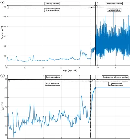
Figure 2.(a)Used accumulation-rate input time series divided in a Holocene and a spin-up section, with time resolution in the Holocene section (20 to 10 520 years b2k) of 1 year. The time resolution for the transition between the Holocene and the spin-up section (10 520 to 12 000 years b2k) is 1 year as well. This is in opposition to the rest of the spin-up section which has a time resolution of 20 years. (b) Surface-temperature spin-up calculated fromδ18Oice calibration. Time resolution equals the accumulation-rate spin-up section. The first-guess surface temperature input is simply a constant value.

This is needed to insure synchroneity between the high-frequency temperature variations 1T(t) extracted from the mismatchD_δ15_N

mc,fin(t) on the ice-age scale and the smooth

temperature solution Tmc,fin(t). Additionally, the signal is

shifted by about 10 years towards modern values to ac-count for gas diffusion from the surface to the lock-in depth (Schwander et al., 1993), which is not yet implemented in the firn model. This is necessary for adding the calculated short-term temperature changes1T(t) to the smooth signal

Tmc,fin(t). The1T values are calculated according to Eq. (3):

1Ti= D_δ15_N

mc,fin,i

N₂,i

, (3)

using the thermal-diffusion sensitivity N2,i for

N2,i=

8.656 ‰

Ti

−1232 ‰·K T2_i

. (4)

Ti is the mean firn temperature in Kelvin which is calculated by the firn model for each time pointi. To reconstruct the fi-nal (high-frequency) temperature input (Thf(t)), the extracted short-term temperature signal1T(t) is simply added to the long-term temperature inputTmc,fin(t):

Thf,i=Tmc,fin,i+1Ti. (5)

2.1.4 Step 4: final correction of the surface temperature solution

For a further improvement of the remainingδ15N and result-ing surface-temperature misfits (D_δ15_N

hf(t),DThf(t)), it is

im-portant to find a correction method that contains information that is also available when using measured data. The bene-fit of the synthetic data study is that several later-unknown quantities can be calculated and used for improving the re-construction approach (see Sects. 3 and 4). For instance, it is possible to split the synthetic δ15Nsyn data in the

gravi-tational and thermodiffusion parts or to use the temperature misfit, which is unknown in reality. The idea underlying the correction algorithm explained hereafter is that the remain-ing misfits ofδ15N (D_δ15_N

hf(t)) and temperature (DThf(t)) are

connected to the Monte Carlo (step 2) and high-frequency part (step 3) of the reconstruction algorithm. In the present inversion framework, it is not possible to find a long-term solutionδ15Nmc,fin(orTmc,fin) which exactly passes through

theδ15Nsyn (orTsyn) target in the middle of the variance in

all parts of the time series. This leads to a slight over- or un-derestimation ofδ15Nmc,fin(t) and their corresponding

tem-perature values Tmc,fin(t). For example, a slightly too low

(or too high) smooth temperature estimate Tmc,fin leads to

a small increase (or decrease) of the firn-column height, cre-ating a wrong gravitational background signal in δ15Nmc,fin

on a later point in time (because the firn column needs some time to react). An additional error in the thermal-diffusion signal is also created due to the high-frequency part of the reconstruction (step 3), because the high-frequency informa-tion is directly extracted from the deviainforma-tion of the synthetic targetδ15Nsyn(t) and the modelledδ15Nmc,fin(t) from the

fi-nal long-term solution Tmc,fin(t) of the Monte Carlo part.

Therefore, this error is transferred into the next step of the reconstruction and partly creates the remaining deviations.

To investigate this problem, the deviationsD_δ15_N

mc,fin(t) of

the synthetic target dataδ15Nsyntoδ15Nmc,fin of the Monte

Carlo part are numerically integrated over a time window of 200 years (Sect. 4, Supplement Sect. S3), and thereafter the window is shifted from past to future in 1-year steps resulting in a time series called IF(t). IF(t) equals a 200-year running mean ofD_δ15_N

mc,fin(t). For t, the middle position of the

win-dow is allocated. The time evolution of IF(t) is a measure

for the deviation of the long-term solutionδ15Nmc,fin(t) (or Tmc,fin(t)) from the perfect middle passage through the

tar-get dataδ15Nsyn(t) (orTsyn(t)) and for the slight over- and

underestimation of the resulting temperature.

IF (t)= 1

200 t+100

Z

t−100

δ15Nsyn(t)−δ15Nmc,fin(t)

dt

= 1

200 t+100

Z

t−100 D_δ15_N

mc,fin(t)dt (6)

Next, the sample cross-correlation function (xcf) (Box et al., 1994) is applied to IF(t) and the remaining misfitsD_δ15_N

hf(t)

of δ15N after the high-frequency part. The xcf shows two extrema (Fig. 3a), a maximum (xcfmax) and a minimum

(xcfmin) at two certain lags (lagmax,δ15_N at xcf_max,δ15_N and

lag_min,δ15_N at xcf_min,δ15_N). Now, the same analysis is

con-ducted for IF(t) versus the temperature mismatch DThf(t)

(Fig. 3b), which shows an equal behaviour (two extrema, lagmax,T at xcfmax,T and lagmin,T at xcfmin,T). Comparing the two cross correlations shows that lag_max,δ15_N equals the

negative lagmin,T and lagmin,δ15_Ncorresponds to the negative

lagmax,T (Fig. 3d, e). The idea for the correction is that the extrema in the cross-correlation IF(t) versusD_δ15_N

hf(t) with

the positive lag (positive means here thatD_δ15_N

hf(t) has to

be shifted to past values relative to IF(t)) creates the mis-fit of temperature DThf(t) on the negative lag (modern

di-rection) of IF(t) versus DThf(t), and vice versa. So, IF(t)

yields information about the cause and allows us to cor-rect this effect between the remaining mismatches,D_δ15_N

hf(t)

and DThf(t), over the whole time series. The lags are not

sharp signals, due to the fact that (i) the cross correlations are conducted over the whole analysed record, leading to an averaging of this cause-and-effect relationship and that (ii) IF(t) is a smoothed quantity itself. The correction of the reconstructed temperature after the high-frequency part is conducted in the following way: from the two linear re-lationships between IF(t) and D_δ15_N

hf(t) at the two lags

(lag_max,δ15_N at xcf_max,δ15_N, lag_min,δ15_N at xcf_min,δ15_N), two

sets ofδ15N correction values (1δ15Nmax(t) from xcfmax,δ15_N

and1δ15Nmin(t) from xcfmin,δ15_N) are calculated. Then, the

lags are inverted (Fig. 3c, e), shifting the two sets of the

δ15N correction values to the attributed lags of the cross correlation between IF(t) and DThf(t) (e.g. 1δ

15_N

min(t) to

lag from xcfmax,T from the cross correlation between IF(t) and DThf(t)), therefore changing the time assignments of

1δ15Nmin(t) and 1δ15Nmax(t) to 1δ15Nmin(t+lagmax,T) and 1δ15Nmax(t+lagmin,T). Now, the 1δ15Nmax(t) and 1δ15Nmin(t) are summed up component-wise, leading to the

time series1δ15Ncv(t). From Eq. (3) with1δ15Ncv,iinstead ofD_δ15_N

mc,fin,i, the corresponding temperature correction val-ues are calculated and added to the high-frequency tempera-ture solutionThf(t), giving the corrected temperatureTcorr(t).

(a) (b)

(c) (d) (e)

Figure 3.Scenario S1:(a)cross-correlation function (xcf) between IF(t) and the remaining mismatch inδ15N (D_δ15_N

hf(t)), after the

high-frequency part shows two extrema: the maximum correlation (max xcf) and the minimum correlation (min xcf).(b)Cross-correlation function (xcf) between IF(t) and the remaining mismatch in temperature (DThf(t)), after the high-frequency part, shows two extrema: the maximum

correlation (max xcf) and the minimum correlation (min xcf).(c)Inverting of panel(a)inx(lag) andy(correlation coefficient) direction. (d)Comparison between panels(a)and(b).(e)Comparison between panels(a)and(c). The temperature-correction values are calculated from the linear dependency between IF(t) andD_δ15_N

hf(t). After shifting IF(t) to max xcf (lag max) and to min xcf (lag min),1δ

15_N max(t) and1δ15Nmin(t) are calculated. Next,1δ15Nmax(t) and1δ15Nmin(t) are inverted. That means, for1δ15Nmax(t), the values are shifted back (−lag max) and shifted further to lag min. After inverting,1δ15Nmax(t) and1δ15Nmin(t) are summed up component-wise to calculate

1δ15Ncv(t). Using1δ15Ncv(t) in Eq. (3) leads to the temperature-correction values which are added to the temperatureThf.

correctedδ15Ncorr(t) time series. This cause-and-effect

rela-tionship found in the cross correlations between IF(t) and

D_δ15_N

hf(t), and IF(t) and DThf(t), is exemplarily shown in

Fig. 3 for scenario S1 and was found for all eight synthetic scenarios. The derived correction algorithm leads to a fur-ther reduction of the mismatches of about 40 % inδ15N and temperature (see Sect. 3.2).

2.2 Firn-densification and heat-diffusion model

Surface-temperature reconstruction relies on firn densifica-tion combined with gas and heat diffusion (Severinghaus et al., 1998). In this study, the firn-densification and heat-diffusion model, developed by Schwander et al. (1997), is used to reconstruct firn parameters for calculating synthetic

δ15N values depending on the input time series. It is a semi-empirical model based on the work of Herron and Lang-way (1980) and Barnola et al. (1991), and implemented us-ing the Crank and Nicholson algorithm (Crank, 1975), and was also used for the temperature reconstructions by Hu-ber et al. (2006) and Kindler et al. (2014). Besides surface-temperature time series, accurate accumulation-rate data are needed to run the model. The model then calculates the den-sification and heat-diffusion history of the firn layer and pro-vides parameters for calculating the fractionation of the ni-trogen isotopes for each time step, according to the following

equations:

δ15Ngrav(zLID, t)=

e

1m·g·z_LID(t)

R·T(t) ₁

·1000 (7)

δ15Ntherm(t)=

_Tsurf(t) Tbottom(t)

αT

−1

·1000 (8)

δ15Nmod(t)=δ15Ngrav(t)+δ15Ntherm(t). (9)

δ15Ngrav(t) is the component of the isotopic fractionation

due to the gravitational settling (Craig et al., 1988; Schwan-der, 1989) and depends on the lock-in depth (LID)zLID(t)

and the mean firn temperature T(t) (Leuenberger et al., 1999).gis the gravitational acceleration,1mthe molar mass difference between the heavy and light isotopes (equal to 10−3kg mol−1 for nitrogen) and R the ideal gas constant.

zLIDis defined as a density thresholdρLID, which is slightly sensitive to surface temperature, following the formula from Martinerie et al. (1994), with a small offset correction of 14 kg m−3to account for the presence of a non-diffusive zone (Schwander et al., 1997):

ρ_LID(kg m−3)= 1 1

ρice−6.95·10

−7_{·T−4.3·10}−5−14, (10)

where

ρice(kg m−3)=916.5−0.14438·T−1.5175·10−4·T 2

The thermal-fractionation component of the δ15N signal (Severinghaus et al., 1998) is calculated using Eq. (8), where

Tsurf(t) and Tbottom(t) stand for the temperatures at the top and the bottom of the diffusive firn layer. In contrast to

Tsurf(t), which is an input parameter for the model,Tbottom(t)

is calculated by the model for each time step. The thermal-diffusion constantαT was measured by Grachev and Sever-inghaus (2003) for nitrogen (Eq. 12):

αT =

8.656−1323K T

·10−3. (12)

The firn model used here behaves purely as a forward model, which means that for the given input time series the output parameters (here, finallyδ15Nmod(t)) can be calculated, but it

is not easily possible to construct from measured isotope data the related surface-temperature or accumulation-rate histo-ries. The goal of the presented study is an automatization of this inverse-modelling procedure for the reconstruction of the rather small Holocene temperature variations.

2.3 Measurement, input data and timescale 2.3.1 Timescale

For the entire study, the GICC05 chronology is used (Ras-mussen et al., 2014; Seierstad et al., 2014). During the whole reconstruction procedure, the two input time series (sur-face temperature and accumulation rate) are split into two parts. The first part ranges from 20 to 10 520 years b2k (called the “Holocene section”) and the second one from 10 520 to 35 000 years b2k (“spin-up section”). The entire accumulation-rate input, as well as the spin-up section of the surface-temperature input, remains unchanged during the re-construction procedure.

2.3.2 Accumulation-rate data

Besides surface temperatures, accumulation-rate data are needed to drive the firn model. In this study, we use the original accumulation rates, reconstructed in Cuffey and Clow (1997), produced using an ice-flow model adapted to the Greenland Ice Sheet Project Two (GISP2) location but adapted to the GICC05 chronology (Rasmussen et al., 2008; Seierstad et al., 2014). A detailed description of the adaption procedure can be found in Sect. S1 of the Supplement. The raw accumulation-rate data for the main part of the spin-up section (12 000 to 35 000 years b2k) are linearly interpolated to a 20-year grid and low-pass filtered with a 200-year COP using cubic-spline filtering (Enting, 1987). For the Holocene section (20–10 520 years b2k) and the transition part between Holocene and spin-up section (10 520 to 12 000 years b2k), the raw accumulation-rate data are linearly interpolated to a 1-year grid to obtain equidistant integer point-to-point dis-tances which are necessary for the reconstruction, and to preserve as much information as possible for this time pe-riod (Fig. 2a). Except for these technical adjustments, the

accumulation-rate input remains unmodified, assuming high reliability of these data during the Holocene. The accumu-lation data were reconstructed using annual layer counting, and a thinning model which should lead to maximum rela-tive uncertainty of 10 % for the first 1500 of the 3000 m ice core (Cuffey and Clow, 1997). From the three accumulation-rate scenarios reconstructed in Cuffey and Clow (1997) and adapted here to the GICC05 chronology, the intermediate one is chosen (red curves in Fig. S1 in the Supplement). Since the differences between the scenarios are not important for the evaluation of the reconstruction approach, they are not taken into account for this study.

Additionally, two sensitivity experiments were conducted (see Sect. S2 in the Supplement) in order to investigate (i) the influence of low-pass filtering of the high-resolution accumu-lation rates on the model outputs and (ii) the possible contri-bution of the accumulation-rate variability to theδ15N data during the Holocene. The first experiment shows that filter-ing the accumulation rates with cut-off periods in the range of 20 to 500 years has nearly no influence on the modelled

δ15N or lock-in depth as long as the major trends are being conserved. The second experiment leads to the finding that the accumulation-rate variability explains about 12 to 30 % ofδ15N variability. A total of 30 % corresponds to the 8.2 kyr event and 12 % to the mean of the whole Holocene period including the 8.2 kyr event. Hence, the influence of accumu-lation changes, excluding the extreme 8.2 kyr event, is gen-erally below 10 % during most parts of the Holocene.

2.3.3 δ18Oicedata

Oxygen-isotope data from the GISP2 ice-core-water sam-ples measured at the University of Washington’s Quater-nary Isotope Laboratory are used to construct the surface-temperature input of the model spin-up (12 to 35 kyr b2k, Grootes et al., 1993; Grootes and Stuiver, 1997; Meese et al., 1994; Steig et al., 1994; Stuiver et al., 1995; data availability: Grootes and Stuiver, 1999). The rawδ18Oicedata are filtered

and interpolated in the same way as the accumulation-rate data for the spin-up part.

2.3.4 Surface-temperature spin-up

The surface-temperature history of the spin-up section (Fig. 2b) is obtained by calibrating the filtered and inter-polatedδ18Oice data (Eq. 13) using the values for the

tem-perature sensitivityα18O and offsetβ found by Kindler et al. (2014) for the North Greenland Ice Core Project (NGRIP) ice core assuming a linear relationship ofδ18Oice with

tem-perature.

Tspin(t)= 1 α18_O(t)

·hδ18Oice(t)+35.2 ‰ i

The values 35.2 ‰ and−31.4◦C are modern-time parame-ters for the GISP2 site (Grootes and Stuiver, 1997; Schwan-der et al., 1997). The spin-up is needed to bring the firn model to a well-defined starting condition that takes possible mem-ory effects (influence of earlier conditions) of firn states into account.

2.3.5 Generating synthetic target data

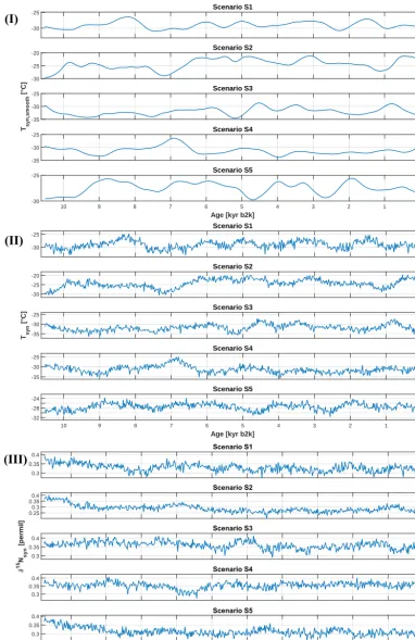
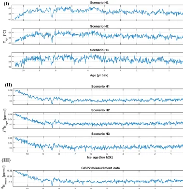
In order to develop and evaluate the presented algorithm, eight temperature scenarios were constructed and used to model synthetic δ15N data, which serve later as targets for the reconstruction. From these eight synthetic surface-temperature and relatedδ15N scenarios (S1–S5 and H1–H3), three datasets (later called Holocene-like scenarios H1–H3) were constructed in such a way that the resultingδ15N time series are very close to theδ15N values measured by Kobashi et al. (2008b) in terms of variability (amplitudes) and fre-quency (data resolution) of the GISP2 nitrogen-isotope data (Figs. 4, 5).

The synthetic surface-temperature scenarios S1–S5 are created by generating a long-term temperature time series (Tsyn,smooth) analogous to the Monte Carlo part of the

recon-struction procedure for only one iteration step (see Sect. 2.1). The values for the cut-off period used for the filtering of the random values, and the SD values (standard deviation of the random values; see Sect. 2.1) for the first five scenarios can be found in Table 3. The long-term temperatures (Fig. 4I) are calculated on a 20-year grid, which is nearly similar to the time resolution of the GISP2 δ15N measurement values of about 17 years (Kobashi et al., 2008b). For the Holocene-like scenarios, the smooth temperature time series were generated from the temperature reconstruction for the GISP2δ15N data (not shown here). The final Holocene surface-temperature solution was filtered with a 100-year cut-off to obtain the long-term temperature scenario.

Following this, high-frequency information is added to the long-term temperature histories. A set of normally dis-tributed random numbers with a zero mean and a standard deviation (1σ) of 1 K for scenarios S1–S5 and 0.3 K for Holocene-like scenarios H1–H3 is generated on the same 20-year grid and added up to the long-term temperature time series. Finally, the resulting synthetic target-temperature sce-narios (Figs. 4II, 5I) are linearly interpolated to a 1-year grid. These synthetic temperatures are combined with the spin-up temperature and are used together with the accumulation-rate input to feed the firn model. From the model out-put, the synthetic δ15N targets are calculated according to Sect. 2.2. The firn-model output provides ice-age as well as gas-age information. The final syntheticδ15N target time se-ries (δ15Nsyn) are set intentionally on the ice-age scale to

mir-ror measured data, because no prior information is available for the gas-age – ice-age difference (1age) for ice-core data.

Table 3.Cut-off periods (COPs) and SD values used for creating the smooth synthetic temperature scenarios according to the Monte Carlo approach.

Scenario COP SD

(years)

S1 1135 0.2065

S2 1007 0.3967

S3 1177 0.4002

S4 1315 0.2952

S5 1244 0.2388

3 Results

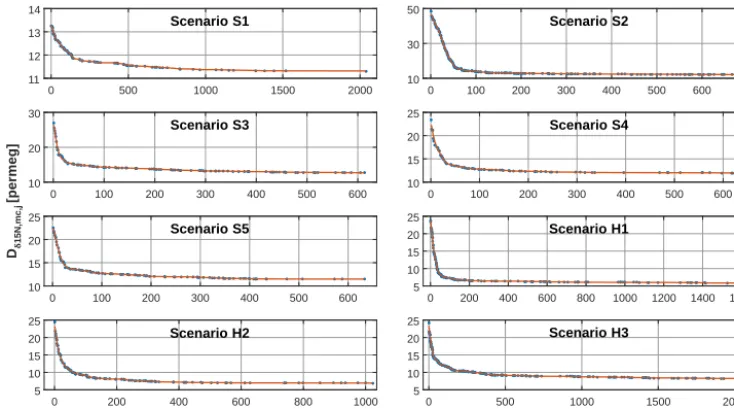
3.1 Monte Carlo type input generator Figure 6 shows the evolution of the misfitD_δ15_N

mc,j between the synthetic target data (δ15Nsyn) and the modelled output δ15Nmc,jof the Monte Carlo part (step 2) as a function of the applied iterations (j) for all synthetic scenarios. One can eas-ily see that all scenarios show a steep decline of the mismatch during the first 50 to 200 iterations followed by a rather mod-erate decrease, which finally leads to a constant value. Dur-ing the Monte Carlo part, it was possible to reduce the mis-fitD_δ15_Nmc compared to the first-guess solutionD_δ15_N

g,0 by

about 15 to 75 % depending on the scenario and the mis-match of the first-guess solution (see Table 2). This leads to a reduction of the temperature mismatchesDTmc compared

to the first-guess temperatureDTg,0 mismatch of about 51 to

87 %.

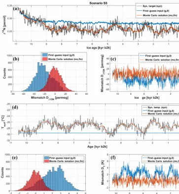
Figure 7 provides the comparison between the first-guess (g,0; step 1) and Monte Carlo (mc,fin; step 2) solution ver-sus the synthetic target data (syn) for the modelled δ15N (Fig. 7a–c) and surface-temperature values (Fig. 7d–f) for scenario S5. Subplots (a) and (d) show the time series of the synthetic target (black dotted line), the first-guess solution (blue line) and the Monte Carlo solution (red line) forδ15N and temperature. In subplots (b) and (e), the distribution of the pointwise mismatchDi of the first-guess (blue) and the Monte Carlo solutions (red) versus the synthetic target data forδ15N (D_δ15_N) and temperature (D_T) can be found.

Sub-plots (c) and (f) contain the time series forD_δ15_N,i andDTi. TheD_δ15_N

mc,fin(t) data (red) are used to calculate the

high-frequency signal that is superimposed to the long-term tem-perature solutionTmc,fin according to Eqs. (3) and (5) (see

Sect. 2.1, step 3). From Fig. 7, it can be concluded that the Monte Carlo part of the reconstruction algorithm (step 2) leads to two major improvements of the first-guess solution. First, it is obvious that the Monte Carlo approach corrects the offsets of the first-guess input (g,0), which shifts the mid-point of the distributions ofD_δ15_N

com--30 -25

Scenario S1

-30 -25 -20

Scenario S2

Tsy

n

[

°C

]

-35 -30 -25

Scenario S3

-35 -30 -25

Scenario S4

Age [kyr b2k]

0 1 2 3 4 5 6 7 8 9 10 -32 -28 -24

Scenario S5

-30

-25 Scenario S1

-30 -25

-20 Scenario S2

Tsy

n,

s

m

oot

h

[

°C

]

-35 -30

-25 Scenario S3

-35 -30

-25 Scenario S4

Age [kyr b2k]

0 1 2 3 4 5 6 7 8 9 10 -30

-25 Scenario S5

(I)

(II)

(III)

-30 -28 -26

Scenario H1

Ts

y

n

[

°C

]

-30 -28 -26

Scenario H2

Age [yr b2k]

0 1 2 3 4 5 6 7 8 9 10 -30 -28 -26

Scenario H3

(I)

(II)

(III)

Figure 5.(I) Synthetic target surface-temperature scenarios H1–H3. (II) Corresponding syntheticδ15N target time series H1–H3. (III) GISP2

δ15N measured data (Kobashi et al., 2008b).

pared to the first guess due to the middle passage through theδ15Nsyntargets. These improvements can be observed for

all eight synthetic scenarios, showing the robustness of the Monte Carlo part (see Table 2, Fig. 7).

3.2 High-frequency step and final correction

Figure 8 provides the comparison between the Monte Carlo (mc,fin; step 2), the high-frequency (hf; step 3) and the cor-rection (corr; step 4) parts of the reconstruction procedure for the scenario S5. Additional data for all other scenarios can be found in Table 4. The upper four plots (Fig. 8a–d) illus-trate each reconstruction step and their effect on the mod-elledδ15N; the bottom four plots (Fig. 8e–h) show the corre-sponding results on the temperature. Plots (a) and (e) contain the time series of the syntheticδ15Nsyn or Tsyntarget (syn;

black dotted line), the high-frequency solution (hf; blue line)

and the final solution after the correction part (corr; red line). For visibility reasons, subplots (b) and (f) display a zoom-in for a randomly chosen time window of about 500 years for the same quantities, which shows the excellent agreement in timing and amplitudes of the modelledδ15N and temperature compared to the synthetic target data. Histograms (c) and (g) and subplots (d) and (h) show the distribution and the time series of the pointwise mismatches (D_δ15_N

iforδ

15_N;D Ti for temperature) between the modelled and the synthetic target data inδ15N and temperature for each reconstruction step.

Compared to the Monte Carlo solution, the high-frequency part leads to a large refinement of the reconstructions. For the meanδ15N misfitsD_δ15_N, the improvement between the

No. of iterations (j)

Dδ

15N,mc

,j

[permeg]

0 500 1000 1500 2000 11

12 13 14

Scenario S1

0 100 200 300 400 500 600 700 10

30 50

Scenario S2

0 100 200 300 400 500 600 10

20 30

Scenario S3

0 100 200 300 400 500 600 10

15 20 25

Scenario S4

0 100 200 300 400 500 600 10

15 20 25

Scenario S5

0 200 400 600 800 1000 1200 1400 1600 5

10 15 20 25

Scenario H1

0 200 400 600 800 1000 5

10 15 20 25

Scenario H2

0 500 1000 1500 2000 5

10 15 20 25

Scenario H3

Figure 6.Evolution of the mean misfit (D_δ15_N

mc) of the modelledδ

15_N

mcversus synthetic targetδ15Nsynas function of the number of iterations (j) for the Monte Carlo approach for all synthetic target scenarios.

Table 4.Summary for the high-frequency (hf) and correction part (corr) of the reconstruction approach.Dis the mean mismatch between the modelledδ15N (or temperature) data and the syntheticδ15N (or temperature) target.σ is the standard deviation of the pointwise mismatches

Di. The 95 % quantiles (2σδ15_N

corr,95 or 2σTcorr,95) of the pointwiseδ

15_{N (or temperature) mismatches are used as an estimate for the 2σ} uncertainty for the final solution (values in bold).

Scenario S1 S2 S3 S4 S5 H1 H2 H3

D_δ15_N

hf(permeg) 2.7 3.6 4.3 3.2 3.5 2.1 2.5 2.6

Improvement (hf vs. MC) (%) 76.1 71.0 66.1 73.1 69.6 63.8 63.8 68.3

σ_δ15_N

hf(permeg) 3.5 4.6 5.4 4.0 4.3 2.7 3.1 3.3

D_δ15_N

corr(permeg) 1.7 2.1 2.6 1.9 2.0 1.2 1.3 1.6

Improvement (corr vs. hf) (%) 37.0 41.7 39.5 40.6 42.9 42.9 48.0 38.5

σ_δ15_N

corr(permeg) 2.2 2.7 3.3 2.4 2.5 1.5 1.7 1.9

2σ_δ15_N

corr,95(permeg) 4.4 5.3 6.3 4.7 4.9 3.0 3.4 3.7

DThf (K) 0.20 0.32 0.33 0.25 0.27 0.18 0.21 0.22

σThf(K) 0.26 0.40 0.43 0.32 0.35 0.22 0.26 0.27

DTcorr (K) 0.12 0.18 0.20 0.14 0.15 0.10 0.11 0.12

σTcorr(K) 0.15 0.24 0.25 0.19 0.19 0.12 0.14 0.15

2σTcorr,95(K) 0.31 0.48 0.51 0.38 0.37 0.23 0.27 0.30

inδ15N and temperature after the high-frequency parts are in the range of about 2.7 to 5.4 permeg (one permeg equals 10−6) forδ15N and 0.22 to 0.40 K for the reconstructed tem-peratures depending on the scenario, which is clearly visible in the decreasing width of the histograms (Fig. 8c and g, blue against grey).

The mismatches after the correction part of the reconstruc-tion approach show clearly a further decrease of the misfits. This means that the width of the distributions of the point-wise mismatches D_δ15_N

i as well asDTi is further reduced, and the distributions become more symmetric (long tales dis-appear; see histograms c and g; red against blue of Fig. 8). The time series of the mismatches (Fig. 8d and h) clearly

illustrate that the correction approach mainly tackles the ex-treme deviations (sharp reduction of exex-treme values’ occur-rence in the red distribution compared to the blue distribu-tion) leading to a further improvement of about 40 % inδ15N and temperature. Finally, the 95 % quantiles (2σ_δ15_N

corr,95,

2σTcorr,95) of the remaining pointwise mismatches ofδ

15_{N and}

temperature (D_δ15_N

measure-Figure 7.(a–c)First-guess (g,0) versus Monte Carlo (mc,fin)δ15N solution for the scenario S5:(a)synthetic targetδ15Nsyn(black dotted line), modelledδ15N time series for the first-guess input (blue line) and Monte Carlo solution (red line).(b)Histogram shows the pointwise mismatches ofD_δ15_Nfor the first-guess solution (blue) and the Monte Carlo solution (red) versus the synthetic target.(c)Time series of

the pointwise mismatches ofD_δ15_Nfor the first-guess solution (blue) and the Monte Carlo solution (red) versus the synthetic target.(d–

f)First-guess versus Monte Carlo surface-temperature solutionTsurffor the scenario S5:(d)synthetic surface-temperature targetTsyn(black dotted line), first-guess temperature input (blue line) and Monte Carlo solution (red line).(e)Histogram shows the pointwise temperature mismatchesDTfor the first-guess solution (blue) and the Monte Carlo solution (red) versus the synthetic surface-temperature target.(f)Time series of the pointwise temperature mismatchesDT for the first-guess solution (blue) and the Monte Carlo solution (red) versus the synthetic surface-temperature target.

ments are of the same order of magnitude, i.e. 3 to 5 permeg (Kobashi et al., 2008b), highlighting the effectiveness of the presented fitting approach. Table 5 contains the final mis-matches (2σ) in1age between the synthetic target and the final modelled data after the correction step for all scenarios, and shows that with a known accumulation rate and assumed perfect firn physics, it is possible to fit the 1age history in the Holocene with mean uncertainties better than 2 years. In other words, the uncertainty in 1age reconstruction due to the inversion algorithm alone is of the order of 2 years.

4 Discussion

4.1 Monte Carlo type input generator

Figure 8.(a–d)δ15N:(a)synthetic targetδ15Nsyn(black dotted line), modelledδ15N time series after adding high-frequency information (hf, blue line) and correction (corr, red line) for the scenario S5.(b)Zoom-in for a randomly chosen 500-year interval shows the decrease of the mismatch after the correction compared to the high-frequency solution.(c)Histogram shows the pointwise mismatchesD_δ15_N of

the synthetic targetδ15Nsynversus the Monte Carlo solution (mc,fin; grey), the high-frequency solution (hf; blue) and the correction (corr; red). The 95 % quantile is 4.9 permeg (yellow line) and used as an estimate for 2σ uncertainty of the final solution.(d)Time series of the pointwise mismatchesD_δ15_N of the synthetic targetδ15Nsynversus the high-frequency solution (hf; blue) and the correction (corr; red).

(e–h)Temperature:(e)synthetic temperature targetTsyn(black dotted line), modelled temperature time series after adding high-frequency information (hf; blue line) and correction (corr; red line).(f)Zoom-in for a randomly chosen 500-year interval shows the decrease of the mismatch after the correction compared to the high-frequency solution.(g)Histogram shows the pointwise mismatchesD_T of the synthetic temperature targetTsynversus the Monte Carlo solution (mc,fin; grey), the high-frequency solution (hf; blue) and the correction (corr; red). The 95 % quantile is 0.37 K (yellow line) and used as an estimate for 2σ uncertainty of the final solution.(h)Time series for the pointwise mismatchesDT of the synthetic temperature targetTsynversus the high-frequency solution (hf; blue) and the correction (corr; red).

used to create the improvements, which implies that itera-tions with small perturbaitera-tions will more likely lead to an im-provement than larger ones.

Figure 6 reveals a weak point of the Monte Carlo part, namely the absence of a suitable termination criterion for the optimization. The implementation until now is conducted

Figure 9.(I) Counts of the COPs and (II) counts of the SD values used to create the improvements for the smooth temperature solutions of the Monte Carlo input generator for all synthetic scenarios (S1–S5 and H1–H3). A SD value of 0.1, for example, means that the maximum allowed perturbation of one temperature valueT(t0) is±10 %.

Table 5.Final mismatches1(1age) (2σ) of1age between the cor-rected solution and the synthetic targets for all scenarios.

Scenario 2σ 1(1age) Scenario 2σ 1(1age)

(yr) (yr)

S1 1.14 S5 1.24

S2 1.60 H1 1.23

S3 1.98 H2 1.18

S4 1.41 H3 1.30

part to about 10 h (a single iteration needs about 90 s). Since the goal of the Monte Carlo part is to find a temperature re-alization that leads to an optimal middle passage through the

δ15N target data, it would be possible to use the mean

dif-ference between theδ15N target and spline-filteredδ15N data using a certain cut-off period as a termination criterion. This issue is under investigation at the moment. Another possi-bility to decrease the time needed for the Monte Carlo part could be an increase in the number of CPUs used for the par-allelization of the model runs. For this study, an eight-core parallelization was used. A further increase in numbers of workers would improve the speed of the optimization.

4.2 High-frequency step and final correction

Sect. S3 in the Supplement). The experiments led to equal results. The major fraction of the final mismatches ofδ15N emerges from mismatches in the thermal-diffusion compo-nentD_δ15_N

therm. Also a cancellation effect between the

grav-itational componentD_δ15_N

gravandDδ15Ntherm of the total

mis-match inδ15N became obvious, affecting the calculation of lag_max,δ15_Nand lag_min,δ15_Nand most likely leading to a

fun-damental residual uncertainty in the low-permeg level for the correctedδ15N data. The same analyses were conducted for all synthetic scenarios, leading to similar results.

Additionally, the influence of the window length, used for the calculation of IF(t), on the correction was analysed, showing that for all investigated window lengths the cor-rection reduces the mismatches of δ15N and temperature, whatever correction mode was used (calculated with xcfmax,

xcfminor both quantities). Moreover, the correction is most

efficient for window lengths in the range of 100 years to 300 years with an optimum at 200 years for all cases.

4.3 Key points to be considered for the application to real data

4.3.1 Benefits of the novel gas-isotope fitting approach In addition to the fitting ofδ15N data, the algorithm is able to fit δ40Ar andδ15Nexcess data as well using the same

ba-sic concepts (Fig. 10). Here, the δ40Ar andδ15Nexcess data

from Kobashi et al. (2008b) were used as the fitting targets. We reach final mismatches (2σ) of 4.0 permeg forδ40Ar/4 and 3.7 permeg for δ15Nexcess, which are for both

quanti-ties below the analytical measurement uncertainty of 4.0 to 9.0 permeg forδ40Ar/4 and 5.0 to 9.8 permeg forδ15Nexcess

measured data (Kobashi et al., 2008b).

The automated inversion of different gas-isotope quanti-ties (δ15N,δ40Ar,δ15Nexcess) provides a unique opportunity

to study the differences in the gained solutions using different targets and to improve our knowledge about the uncertain-ties of gas-isotope-based temperature reconstructions using a single firn model. Next, the presented algorithm is not de-pendent on the firn model, which leads to the implication that the algorithm can be coupled to different firn models describ-ing firn physics in different ways. Furthermore, an automated reconstruction algorithm avoiding manual manipulation and leading to reproducible solutions makes it possible for the first time, to study and learn from the differences between solutions matching different targets. Finally, differences ob-tained by applying different firn physics (densification equa-tions, convective zone, etc.) but the very same inversion algo-rithm may help to assess firn-model shortcomings, resulting in more robust uncertainty estimates than it was ever possible before.

In this publication, we show the functionality and the basic concepts of the automated inversion algorithm using well-known synthetic δ15N fitting targets. In this “perfect-world scenario”, the forward problem, converting surface

tempera-ture toδ15N, as well as the inverse problem, convertingδ15N to surface temperature, are completely described by the used firn model. Consequently, all sources of signal noise are ig-nored. For the later use of the algorithm on δ15N, δ40Ar or δ15Nexcess measured data, this will not be the case

any-more due to different sources of signal noise in the used measured data. As a result, differences between tempera-ture solutions obtained from individual targets (δ15N,δ40Ar,

δ15Nexcess) will become obvious. These differences will

al-low us to quantify the uncertainties associated with different unconstrained processes. Next, we will list and discuss po-tential sources of uncertainties and try to provide suggestions for their handling and quantification in our approach.

4.3.2 Measurement uncertainty and firn heterogeneity (centimetre-scale variability)

Many studies have investigated the influence of firn het-erogeneity (or density fluctuations) on measurements of air compounds and quantities (e.g. δ15N, δ40Ar, CH4, CO2,

O2/N2ratio, air content) extracted from ice cores resulting

uncer-M M

M M

Figure 10.Fitting of GISP2 Holoceneδ40Ar(a–d)andδ15Nexcess(e–h)data (measurement data from Kobashi et al., 2008b):(a)measured versus modelledδ40Ar/4 time series.(b)Zoom-in for the same quantity as in panel(a).(c)Time series of the final mismatches1δ40Ar/4 of the measured minus the modelledδ40Ar/4 data.(d)Histogram for the same quantity as in panel(c)showing an overall final mismatch (2σ) of 4.0 permeg and offset (os) of−0.5 permeg.(e)Measured versus modelledδ15Nexcesstime series.(f)Zoom-in for the same quantity as in panel(e).(g)Time series of the final mismatches1δ15Nexcessof the measured minus the modelledδ15Nexcessdata.(h)Histogram for the same quantity as in panel(g)showing an overall final mismatch (2σ) of 3.7 permeg and offset (os) of−0.8 permeg.

tainty in the inverse-modelling approach presented here. This will increase the uncertainty of the temperature according to Eq. (3).The same equation can also be used for the calcula-tion of the uncertainty in temperature related to measurement uncertainty in general.

To answer the pertinent question of how to better extract a meaningful temperature history from a noisy ice-core record, an excellent – but costly – solution is of course to use multi-ple ice cores. For exammulti-ple, aδ15N-based temperature recon-struction from the combination of data from the GISP2 ice core with the “sister ice core” GRIP drilled 30 km apart is likely one of the best ways to overcome potential

centimetre-scale variability. A comparison of ice cores that were drilled even closer might be even more advantageous.

4.3.3 Smoothing effects due to gas diffusion and trapping

(Schwan-der et al., 1997), whereas the data resolution of the synthetic targets was set to 20 years to mimic the measurement data from Kobashi et al. (2008b) with a mean data resolution of about 17 years (see Sect. 2.3: “Generating synthetic target data”). In the study of Kindler et al. (2014), it was shown that a glacial Greenland lock-in depth leads to a damping of theδ15N signal of about 30 % for a 10 K temperature rise in 20 years. We further assume that the smoothing according to the lock-in process is negligible for Greenland Holocene conditions according to the much smaller amplitude signals and shallower LID. Yet, for glacial conditions, it requires at-tention.

4.3.4 Accumulation-rate uncertainties

For the synthetic data study presented in this paper, it is as-sumed that the used accumulation-rate data are well known with zero uncertainty. This simplification is used to show the functionality and basic concepts of the presented fitting al-gorithm in every detail on well-known δ15N and tempera-ture targets and to focus on the final uncertainties originating from the presented fitting algorithm itself. For the later re-construction using measured gas-isotope data together with the published accumulation-rate scenarios shown in Sect. S1 of the Supplement, this will not be the case anymore. Un-certainties in layer counting and corrections for ice thinning will lead to a fundamental uncertainty. Especially in the early Holocene, this can easily exceed 10 %. As the accumulation-rate data are used to run the firn model, all potential accumu-lation uncertainties are in part incorporated into the temper-ature reconstruction. On the other hand, as we discussed in Sect. S2 of the Supplement, the accumulation-rate variabil-ity has a minor impact compared to the input temperature on the variability of δ15N data in the Holocene. The influ-ence of these quantities, accumulation rate or temperature, on the temperature reconstruction is not equal; during the Holocene, accumulation-rate variability explains about 12 to 30 % ofδ15N variability. A total of 30 % corresponds to the 8.2 kyr event and 12 % to the mean of the whole Holocene period including the 8.2 kyr event. Hence, the influence of accumulation changes, excluding the extreme 8.2 kyr event, is generally below 10 % during the Holocene. If the accumu-lation is assumed to be completely correct, then the missing part will be assigned to temperature variations. Nevertheless, for the fitting of the Holocene measurement data, we will use all three accumulation-rate scenarios as shown in Sect. S1 of the Supplement. The difference in the reconstructed tempera-tures arising from the differences of these three scenarios will be used for the uncertainty calculation as well and is most likely higher than the uncertainty arising from uncertainties due to the process of producing the accumulation-rate data and from the conversion of the accumulation-rate data to the GICC05 timescale.

4.3.5 Convective zone variability

Many studies have shown the existence of a well-mixed zone at the top of the diffusive firn column, called the con-vective zone (CZ). The CZ is formed by strong katabatic winds and pressure gradients between the surface and the firn (e.g. Kawamura et al., 2006, 2013; Severinghaus et al., 2010). The existence of a CZ changes the gravitational back-ground signal inδ15N andδ40Ar as it reduces the diffusive-column height. The presented fitting algorithm was used to-gether with the two most frequently used firn models for tem-perature reconstructions based on stable isotopes of air, the Schwander et al. (1997) model which has no CZ built in (or better – a constant CZ of 0 m) and the Goujon firn model (Goujon et al., 2003) (which assumes a constant convective zone over time, that can easily be set in the code). This differ-ence between the two firn models only changes significantly the absolute temperature rather than the temperature anoma-lies as it was shown by other studies (e.g. Guillevic et al., 2013, Fig. 3). In the presented work, we show the results us-ing the model from Schwander et al. (1997), because the dif-ferences between the obtained solutions using the two mod-els are negligible, except a constant temperature offset. Also noteworthy is that there is no firn model at the moment which uses a dynamically changing CZ. Indeed, this should be in-vestigated but requires additional intense work. Additionally, the knowledge of the time evolution of CZ changes for time periods of millennia to several hundreds of millennia (in fre-quency and magnitude) is too poor to estimate the influence of this quantity on the reconstruction. In principle, it is pos-sible to cancel out the influence of a potentially changing CZ by usingδ15Nexcess data for temperature reconstruction, as

due to the subtraction ofδ40Ar/4 fromδ15N the gravitational term of the signals is eliminated. From that point of view, it will be interesting to compare temperature solutions gained fromδ15Nexcess fitting with the solutions based on δ15N or δ40Ar alone. This can offer a useful tool for quantifying the magnitude and frequency of CZ changes in the time interval of interest.

It is known that for some very low accumulation-rate sites in areas with strong katabatic winds (e.g. “megadunes”, Antarctica) extremely deep CZs can occur, which are po-tentially able to smooth out even decadal-scale temperature variations (Severinghaus et al., 2010). For this, its deepness would need to be of several dozens of metres, which is highly unrealistic even for glacial Summit conditions (Guillevic et al., 2013; see discussion in Annex A4, p. 1042) as well as for the rather stable Holocene period in Greenland for which no low accumulation and strong katabatic wind situations are to be expected.

4.4 Proof of concept for glacial data