SAS LASR Analytic Server 2.4

(1)

SAS

®

LASR

™

Analytic

Server 2.4

Reference Guide

(2)

For a hard-copy book: No part of this publication may be reproduced, stored in a retrieval system, or transmitted, in any form or by any means, electronic, mechanical, photocopying, or otherwise, without the prior written permission of the publisher, SAS Institute Inc.

For a web download or e-book: Your use of this publication shall be governed by the terms established by the vendor at the time you acquire this publication.

The scanning, uploading, and distribution of this book via the Internet or any other means without the permission of the publisher is illegal and punishable by law. Please purchase only authorized electronic editions and do not participate in or encourage electronic piracy of copyrighted materials. Your support of others' rights is appreciated.

U.S. Government License Rights; Restricted Rights: The Software and its documentation is commercial computer software developed at private expense and is provided with RESTRICTED RIGHTS to the United States Government. Use, duplication or disclosure of the Software by the United States Government is subject to the license terms of this Agreement pursuant to, as applicable, FAR 12.212, DFAR 227.7202-1(a), DFAR 227.7202-3(a) and DFAR 227.7202-4 and, to the extent required under U.S. federal law, the minimum restricted rights as set out in FAR 52.227-19 (DEC 2007). If FAR 52.227-19 is applicable, this provision serves as notice under clause (c) thereof and no other notice is required to be affixed to the Software or documentation. The Government's rights in Software and documentation shall be only those set forth in this Agreement.

SAS Institute Inc., SAS Campus Drive, Cary, North Carolina 27513-2414. August 2014

SAS provides a complete selection of books and electronic products to help customers use SAS® software to its fullest potential. For more information about our offerings, visit support.sas.com/bookstore or call 1-800-727-3228.

SAS® and all other SAS Institute Inc. product or service names are registered trademarks or trademarks of SAS Institute Inc. in the USA and other countries. ® indicates USA registration.

(3)

(4)

(5)

What’s New In SAS LASR

Analytic Server

Overview

SAS LASR Analytic Server 2.4 includes the following changes: • Enhancements to the IMSTAT procedure

• Compression for in-memory tables and SASHDAT tables • Enhancements to the RECOMMEND procedure

• Documentation enhancements

Enhancements to the IMSTAT Procedure

The following enhancements have been made to the IMSTAT procedure:

• The AGGREGATE statement is new for the 2.4 release. You can aggregate values of one or more variables and specify the aggregate method to use for each variable. • The CLUSTER statement is enhanced with a CODE option. You can use this option

to save the DATA step scoring code for the clustering.

• The CREATETABLE statement is new. It is used to create an empty in-memory table that is later used for appending records to it. It had been added to support working with event stream processing.

• The FORECAST statement is enhanced to support goal-seeking forecasts. The CONTROLVARS=, UPPER=, and LOWER= options are used to specify the control variables and bounds. The GOAL= option is used to specify the goal variable and the WEIGHT= option is used to specify a weight for the goal variable.

• The GENMODEL statement is enhanced with the VARSELECTION option to support variable selection.

• The GLM statement is enhanced with the VIF option to support computing variable inflation factors and tolerances.

• The HISTOGRAM statement is enhanced with the ROUNDINGDIRECTION= option.

• The SLSTAY= option in the GLM, LOGISTIC, and GENMODEL statements automatically triggers variable selection. In previous releases, you had to specify the VARSELECTION or SHOWSELECTION option to trigger variable selection.

(10)

Compressed In-Memory Tables and SASHDAT

Tables

The server can read and write compressed in-memory tables. You can compress data as you load data to memory as follows:

• The SAS LASR Analytic Server engine is enhanced with a SQUEEZE= option. The server compresses the data as the table is loaded to memory.

• The LASR procedure is enhanced to support a SQUEEZE option. When you specify the option, the server compresses the data as the table is loaded to memory.

When a table is already in-memory, you can compress it with the COMPRESS statement in the IMSTAT procedure.

SASHDAT tables in HDFS can also be compressed. The advantage of compressing tables in HDFS is not to save disk space, but to combine the in-memory table compression with the memory efficiencies of the SASHDAT format. You can use SASHDAT tables with compression as follows:

• The SAS Data in HDFS engine is enhanced with a SQUEEZE= option. The data are compressed as the rows are added to the SASHDAT table in HDFS.

• The SAVE statement for the IMSTAT procedure is enhanced with a SQUEEZE option that saves the in-memory table to HDFS in compressed form.

Enhancements to the RECOMMEND Procedure

The PREDICT statement is enhanced to include a TEMPTABLE option and the ITEMDATA= option.

Enhancements to Data Access

For distributed SAS LASR Analytic Server, the syntax for loading data in parallel from remote data clusters is simplified:

• You no longer need to specify the GRIDDATASERVER= option in the

PERFORMANCE statement or set the GRIDDATASERVER environment variable. • You no longer need to specify the GRIDMODE= option in the PERFORMANCE

statement or set the GRIDMODE environment variable.

This enhancement is common to SAS high-performance procedures. For more information, see "Data Access Modes" in Base SAS Procedures Guide: High-Performance Procedures.

(11)

Documentation Enhancements

The following changes are included in this release:

• The ORDERBYDESC option for the SUMMARY statement of the IMSTAT procedure was incorrectly identified as the ORDERDESC option in previous releases of this document.

• Two examples of the FORECAST statement in the IMSTAT procedure are added. • Information about working with HDFS has been added. See “Common HDFS

Commands” on page 368.

• Information about passwordless SSH has been enhanced and moved to a single section. See “Passwordless SSH” on page 12.

• Information about the IMPORTCUBE statement in the IMSTAT procedure is removed.

(12)

(13)

Chapter 1 Introduction to the SAS LASR

Analytic Server

What is SAS LASR Analytic Server? . . . 2

How Does the SAS LASR Analytic Server Work? . . . 3

Distributed SAS LASR Analytic Server . . . 3

Non-Distributed SAS LASR Analytic Server . . . 4

About the SAS High-Performance Deployment of Hadoop . . . 5

Benefits of Using the Hadoop Distributed File System . . . 5

Components of the SAS LASR Analytic Server . . . 6

About the Components . . . 6

Root Node . . . 6

Worker Nodes . . . 6

In-Memory Tables . . . 6

Signature Files . . . 6

Server Description Files . . . 7

Administering the SAS LASR Analytic Server . . . 7

Administering a Distributed Server . . . 7

Administering a Non-Distributed Server . . . 7

Common Administration Features . . . 8

Features Available in SAS Visual Analytics Administrator . . . 8

Understanding Server Run Time . . . 8

Distributing Data . . . 9

Passwordless SSH . . . 12

What Is Passwordless SSH? . . . 12

Who Needs Passwordless SSH? . . . 12

How to Set Up Passwordless SSH . . . 12

Generate SSH Keys Manually . . . 13

About Passwordless SSH and Windows Clients . . . 13

Troubleshooting . . . 14

Memory Management . . . 14

About Physical and Virtual Memory . . . 14

How Does the Server Use Memory for Tables? . . . 15

How Else Does the Server Use Memory? . . . 15

Managing Memory . . . 15

Data Partitioning and Ordering . . . 16

Overview of Partitioning . . . 16

Understanding Partition Keys . . . 17

Ordering within Partitions . . . 17

SAS LASR Analytic Server Logging . . . 18

(14)

Understanding Logging . . . 18

What is Logged? . . . 18

Log Record Format . . . 18

Data Compression . . . 20

Overview of Data Compression . . . 20

Compressed Tables and the DATA Step . . . 21

Compressed Tables and the LASR Procedure . . . 21

Performance Considerations . . . 22

Interactions . . . 22

Limitations . . . 24

What is SAS LASR Analytic Server?

The SAS LASR Analytic Server is an analytic platform that provides a secure, multi-user environment for concurrent access to data that is loaded into memory. The server can take advantage of a distributed computing environment by distributing data and the workload among multiple machines and performing massively parallel processing. The server can also be deployed on a single machine where the workload and data volumes do not demand a distributed computing environment.

The server handles both big data and smaller sets of data, and it is designed with a high-performance, multi-threaded, analytic code. The server processes client requests at extraordinarily high speeds due to the combination of hardware and software that is designed for rapid access to tables in memory. By loading tables into memory for analytic processing, the server enables business analysts to explore data and discover relationships in data at the speed of RAM.

The server can also perform text analysis on unstructured data. The unstructured data is loaded to memory in the form of a table, with one document in each row. The

TEXTPARSE statement in the IMSTAT procedure can then provide similar analysis to what is available with the HPTMINE procedure.

Another use for the analytic platform that the server provides is to create a recommender system. Creating recommender systems introduces the concept of an application in the server. The recommender system contains the application and might contain four or five tables. Each of the tables can be used in different ways, depending on the task and which method you apply. For example, making an item-based prediction for a nearest-neighbor method requires different data structures than a singular-value decomposition. You can associate a particular method or a set of methods with the application. You can execute one method or an ensemble. The flexibility provided by the server enables you to add and drop methods from the application. As a modeler, you want to explore and evaluate with different methods and different parameter configurations for the methods until you have optimized the system for your purposes. Then, you can deploy the recommender system in an online scoring environment.

The architecture for the server was originally designed for optimal performance in a distributed computing environment. A distributed server runs on multiple machines. A typical distributed configuration is to use a series of blades as a cluster. Each blade contains both local storage and large amounts of memory. Local storage is used to store large data sets in distributed form. Data is loaded into memory and made available so that clients can quickly access that data.

For distributed deployments, having local storage available on machines is critical in order to store large data sets in a distributed form. The server supports the Hadoop Distributed File System (HDFS) as a co-located data provider. HDFS is used because the

(15)

server can read from and write to HDFS in parallel. In addition, HDFS provides replication for data redundancy. HDFS stores data as blocks in distributed form on the blades and the replication provides failover capabilities.

In a distributed deployment, the server also supports some third-party vendor databases as co-located data providers. Teradata Data Warehouse Appliance and Greenplum Data Computing Appliance are massively parallel processing database appliances. You can install the SAS LASR Analytic Server software on each of the machines in either appliance. The server can read in parallel from the local data on each machine. For the SAS LASR Analytic Server 1.6 release (concurrent with the SAS Visual Analytics 6.1 release) the server supports a distributed deployment. A non-distributed server can perform the same in-memory analytic operations as a non-distributed server. However, a non-distributed deployment does not support parallel I/O from HDFS or third-party vendor appliances.

How Does the SAS LASR Analytic Server Work?

Distributed SAS LASR Analytic Server

The server provides a client/server environment where the client connects to the server, sends requests to the server, and receives results back from the server. The server-side environment is a distributed computing environment. A typical deployment is to use a series of blades in a cluster. In addition to using a homogeneous hardware profile, the software installation is also homogeneous. The same operating system is used throughout and the same SAS software is installed on each blade that is used for the server. In order for the software on each blade to share the workload and still act as a single server, the SAS software that is installed on each blade implements the Message Passing Interface (MPI). The MPI implementation is used to enable communication between the blades.

After a client connection is authenticated, the server performs the operations requested by the client. Any request (for example, a request for summary statistics) that is authorized will execute. After the server completes the request, there is no trace of the request. Every client request is executed in parallel at extraordinarily high speeds, and client communication with the server is practically instantaneous and seamless. There are two ways to load data into a distributed server:

• load data from tables and data sets. You can start a server instance and directly load tables into the server by using the SAS LASR Analytic Server engine or the LASR procedure from a SAS session that has a network connection to the cluster. Any data source that can be accessed with a SAS engine can be loaded into memory. The data is transferred to the root node of the server and the root node distributes the data to the worker nodes. You can also append rows to an in-memory table with the SAS LASR Analytic Server engine.

• load tables from a co-located data provider.

• Tables can be read from the Hadoop Distributed File System (HDFS). You can use the SAS Data in HDFS engine to add tables to HDFS. When a table is added to HDFS, it is divided into blocks that are distributed across the machines in the cluster. The server software is designed to read data in parallel from HDFS. When used to read data from HDFS, the LASR procedure causes the worker nodes to read the blocks of data that are local to the machine.

(16)

• Tables can also be read from a third-party vendor database. For distributed databases like Teradata and Greenplum, the SAS LASR Analytic Server can access the local data on each machine that is used for the database.

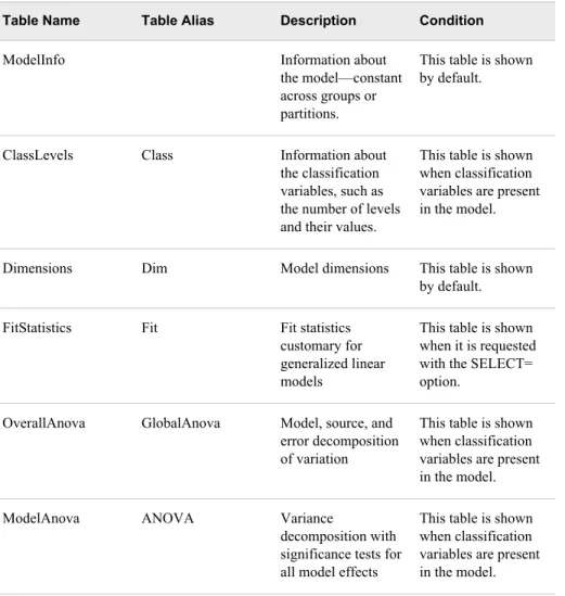
The following figure shows the relationship of the root node, the worker nodes, and how they interact when working with large data sets in HDFS. As described in the previous list, the LASR procedure communicates with the root node and the root node directs the worker nodes to read data in parallel from HDFS. The figure also indicates how the SAS Data in HDFS engine is used to transfer data to HDFS.

Figure 1.1 Relationship of PROC LASR and the SAS Data in HDFS Engine

Root Node PROC LASR

SAS Data in HDFS Engine

Worker Node

Hadoop NameNode

HDFS

SAS Data

HDFS HDFS HDFS

Note: The preceding figure shows a distributed architecture that uses HDFS. For deployments that use a third-party vendor database, the architecture is also distributed, but different procedures and software components are used for distributing and reading the data.

After the data is loaded into memory on the server, it resides in memory until the table is unloaded or the server terminates. After the table is in memory, client applications that are authorized to access the table can send requests to the server and receive the results from the server.

In-memory tables can be saved. You can use the SAS LASR Analytic Server engine to save an in-memory table as a SAS data set or as any other output that a SAS engine can use. This method of using an engine transfers the data across the network connection. For large tables, saving to HDFS is supported with the LASR and IMSTAT procedures. This strategy saves the data in parallel and keeps the data on the cluster.

Non-Distributed SAS LASR Analytic Server

Most of the features that are available with a distributed deployment also apply to the non-distributed deployment too. Any limitations are related to the reduced functionality of using a single-machine rather than a distributed computing environment.

In a non-distributed deployment, the server acts in a client/server fashion where the client sends requests to the server and receives results back. The server performs the analytic operations on the tables that are loaded in to memory. As a result, the processing times are very fast and the results are delivered almost instantaneously.

You can load tables to a non-distributed server with the SAS LASR Analytic Server engine. Any data source that SAS can access can be used for input and the SAS LASR Analytic Server engine can store the data as an in-memory table. The engine also supports appending data.

(17)

You can save in-memory tables by using the SAS LASR Analytic Server engine. The tables can be saved as a SAS data set or as any other output that a SAS engine can use.

About the SAS High-Performance Deployment of

Hadoop

SAS offers the SAS High-Performance Deployment of Hadoop that includes the following:

• Hadoop software that is provided by Apache

• two JAR files that provide services that run inside Hadoop

• an executable file, saslasrfd, that facilitates reading data in parallel into SAS LASR Analytic Server

• an installation program that simplifies installation and configuration on the cluster The JAR files and the executable are installed automatically when you install SAS High-Performance Deployment of Hadoop. As an alternative, you can manually configure several commercially available Hadoop distributions with the JAR files and executable. After you have performed the manual configuration, the commercially available distribution is functionally equivalent to SAS High-Performance Deployment of Hadoop. The cluster then supports parallel I/O with SAS LASR Analytic Server as well as operating with the SAS Data in HDFS engine.

See Also

SAS High-Performance Analytics Infrastructure: Installation and Configuration Guide

Benefits of Using the Hadoop Distributed File

System

Loading data from disk to memory is efficient when the SAS LASR Analytic Server is co-located with a distributed data provider. The Hadoop Distributed File System (HDFS) provided by SAS High-Performance Deployment of Hadoop acts as a co-located data provider. HDFS offers some key benefits:

• Parallel I/O. The SAS LASR Analytic Server can read data in parallel at very impressive rates from a co-located data provider.

• Data redundancy. By default, two copies of the data are stored in HDFS. If a machine in the cluster becomes unavailable or fails, the SAS LASR Analytic Server instance on another machine in the cluster retrieves the data from a redundant block and loads the data into memory.

• Homogeneous block distribution. HDFS stores files in blocks. The SAS implementation enables a homogeneous block distribution that results in balanced memory utilization across the SAS LASR Analytic Server and reduces execution time.

(18)

Components of the SAS LASR Analytic Server

About the Components

The following sections identify some software components and interactions for SAS LASR Analytic Server.

Root Node

When the SAS client initiates contact with the grid host to start a SAS LASR Analytic Server instance, the SAS software on that machine takes on the role of distributing and coordinating the workload. This role is in contrast to a worker node. This term applies to a distributed SAS LASR Analytic Server only.

Worker Nodes

This is the role of the software that receives the workload from the root node. When a table is loaded into memory, the root node distributes the data to the worker nodes and they load the data into memory. If you are using a co-located data provider, each worker node reads the portion of the data that is local to the machine. The data is loaded into memory and requests that are sent to root node are distributed to the worker nodes. The worker nodes perform the analytic tasks on the data that is loaded in memory on the machine and then return the results to the root node. This term applies to a distributed SAS LASR Analytic Server only.

In-Memory Tables

SAS LASR Analytic Server performs analytics on tables that are in-memory only. Typically, large tables are read from a co-located data provider by worker nodes. The tables are loaded quickly because each worker node is able read a portion of the data from local storage. Once the portion of the table is in memory on each worker node, the server instance is able to perform the analytic operations that are requested by the client. The analytic tasks that are performed by the worker nodes are done on the in-memory data only.

Signature Files

SAS LASR Analytic Server uses two types of signature files, server signature files and table signature files. These files are used as a security mechanism for server

management and for access to data in a server. When a server instance is started, a directory is specified on the PATH= option to the LASR procedure. The specified directory must exist on the machine that is specified as GRIDHOST= environment variable.

In order to start a server, the user must have Write access to the directory in order to be able to create the server signature file. In order stop a server, the user must have Read access to the server signature file so that it can be removed from the directory. In order to load and unload tables on a server, the user must have Read access to the server signature file in order to interact with the server. Write permission to the directory

(19)

is needed to create the table signature file when loading a table and to delete the table signature file when unloading the table.

Server Description Files

Note: Most administrators prefer to use the PORT= option in the LASR procedure rather than use server description files.

If you specify a filename in the CREATE= option in the LASR procedure, then you start a SAS LASR Analytic Server instance, the LASR procedure creates two files:

• a server description file

• a server signature file (described in the previous section)

The server description file contains information such as the host names of the machines that are used by the server instance and signature file information.

In the LASR procedure, the server description file is specified with the CREATE= option. The server description file is created on the SAS client machine that invoked PROC LASR.

Administering the SAS LASR Analytic Server

Administering a Distributed Server

Basic administration of a distributed SAS LASR Analytic Server can be performed with the LASR procedure from a SAS session. Server instances are started and stopped with the LASR procedure. The LASR procedure can be used to load and unload tables from memory though the SAS LASR Analytic Server engine also provides that ability. The SAS Data in HDFS engine is used to add and delete tables from the Hadoop Distributed File System (HDFS). The tables are stored in the SASHDAT file format. You can use the DATASETS procedure with the engine to display information about tables that are stored in HDFS.

The HPDS2 procedure has a specific purpose for use with SAS LASR Analytic Server. In this deployment, the procedure is used to distribute data to the machines in an appliance. After the data are distributed, the SAS LASR Analytic Server can read the data in parallel from each of the machines in the appliance.

Administering a Non-Distributed Server

A distributed SAS LASR Analytic Server runs on a single machine. A non-distributed server is started and stopped with the SAS LASR Analytic Server engine. A server is started with the STARTSERVER= option in the LIBNAME statement. The server is stopped when one of the following occurs:

• The libref is cleared (for example, libname lasrsvr clear;). • The SAS program and session that started the server ends. You can use the

SERVERWAIT statement in the VASMP procedure to keep the SAS program (and the server) running.

• The server receives a termination request from the SERVERTERM statement in the VASMP procedure.

(20)

A non-distributed deployment does not include a distributed computing environment. As a result, a non-distributed server does not support a co-located data provider. Tables are loaded and unloaded from memory with the SAS LASR Analytic Server engine only. Common Administration Features

As described in the previous sections, the different architecture for distributed and non-distributed servers requires different methods for starting, stopping, and managing tables with servers. However, the IMSTAT procedure works with distributed and

non-distributed servers to provide administrators with information about server instances. The statements that provide information that can be of interest to administrators are as follows:

• SERVERINFO • TABLEINFO

Administrators might also be interested in the SERVERPARM statement. You can use this statement to adjust the number of requests that are processed concurrently. You might reduce the number of concurrent requests if the number of concurrent users causes the server to consume too many sockets from the operating system.

Features Available in SAS Visual Analytics Administrator

SAS LASR Analytic Server is an important part of SAS Visual Analytics. SAS Visual Analytics Administrator is a web application that provides an intuitive graphical interface for server management. You can use the application to start and stop server instances, as well as load and unload tables from the servers. Once a server is started, you can view information about libraries and tables that are associated with the server. The application also indicates whether a table is in-memory or whether it is unloaded. For deployments that use SAS High-Performance Deployment of Hadoop, an HDFS explorer enables you to browse the tables that are stored in HDFS. Once tables are stored in HDFS, you can to load them into memory in a server instance. Because SAS uses the special SASHDAT file format for the data that is stored in HDFS, the HDFS explorer also provides information about the columns, row count, and block distribution. Understanding Server Run Time

By default, servers are started and run indefinitely. However, in order to conserve the hardware resources in a distributed computing environment, server instances can be configured to exit after a period of inactivity. This feature applies to distributed SAS LASR Analytic Server deployments only. You specify the inactivity duration with the LIFETIME= option when you start the server.

When the LIFETIME= option is used, each time a server is accessed, such as to view data or perform an analysis, the run time for the server is reset to zero. Each second that a server is unused, the run timer increments to count the number of inactive seconds. If the run timer reaches the maximum run time, the server exits. All the previously used hardware resources become available to the remaining server instances.

(21)

Distributing Data

SAS High-Performance Deployment of Hadoop

SAS provides SAS High-Performance Deployment of Hadoop as a co-located data provider. The SAS LASR Analytic Server software and the SAS High-Performance Deployment of Hadoop software are installed on the same blades in the cluster. The SAS Data in HDFS engine can be used to distribute data to HDFS.

For more information, see “Using the SAS Data in HDFS Engine” on page 367. PROC HPDS2 for Big Data

For deployments that use Greenplum or Teradata, the HPDS2 procedure can be used to distribute large data sets to the machines in the appliance. The procedure provides an easy-to-use and efficient method for transferring large data sets.

For deployments that use Greenplum, the procedure is more efficient than using a DATA step with the SAS/ACCESS Interface to Greenplum and is an alternative to using the gpfdist utility.

The SAS/ACCESS Interface for the database must be configured on the client machine. It is important to distribute the data as evenly as possible so that the SAS LASR Analytic Server has an even workload when the data is read into memory.

The following code sample shows a LIBNAME statement and an example of the HPDS2 procedure for adding tables to Greenplum.

libname source "/data/marketing/2012"; libname target greenplm

server = "grid001.example.com" user = dbuser

password = dbpass schema = public database = template1 dbcommit=1000000;

proc hpds2 data = source.mktdata

out = target.mktdata (distributed_by = 'distributed randomly'); 1

performance host = "grid001.example.com" install = "/opt/TKGrid";;

data DS2GTF.out; method run(); set DS2GTF.in; end;

enddata; run;

proc hpds2 data = source.mkdata2

out = target.mkdata2 (dbtype=(id='int') distributed_by='distributed by (id)'); 2

performance host = "grid001.example.com" install = "/opt/TKGrid";

(22)

data DS2GTF.out; method run(); set DS2GTF.in; end;

enddata; run;

1 The rows of data from the input data set are distributed randomly to Greenplum. 2 The id column in the input data set is identified as being an integer data type. The

rows of data are distributed based on the value of the id column.

For information about the HPDS2 procedure, see the Base SAS Procedures Guide: High-Performance Procedures. The procedure documentation is available from http:// support.sas.com/documentation/cdl/en/prochp/66409/HTML/ default/viewer.htm#prochp_hpds2_toc.htm.

Bulkload for Teradata

The SAS/ACCESS Interface to Teradata supports a bulk-load feature. With this feature, a DATA step is as efficient at transferring data as the HPDS2 procedure.

The following code sample shows a LIBNAME statement and two DATA steps for adding tables to Teradata.

libname tdlib teradata server="dbc.example.com" database=hps

user=dbuser password=dbpass bulkload=yes; 1

data tdlib.order_fact; set work.order_fact; run;

data tdlib.product_dim (dbtype=(partno='int') 2

dbcreate_table_opts='primary index(partno)'); 3

set work.product_dim; run;

data tdlib.salecode(dbtype=(_day='int' fpop='varchar(2)') bulkload=yes

dbcreate_table_opts='primary index(_day,fpop)'); 4

set work.salecode; run;

data tdlib.automation(bulkload=yes dbcommit=1000000 5

dbcreate_table_opts='unique primary index(obsnum)'); 6

set automation; obsnum = _n_; run;

1 Specify the BULKLOAD=YES option. This option is shown as a LIBNAME option but you can specify it as a data set option.

(23)

3 Specify to use the variable named partno as the distribution key for the table. 4 Specify to use the variables that are named _day and fpop as a distribution key for

the table that is named salecode.

5 Specify the DBCOMMIT= option when you are loading many rows. This option interacts with the BULKLOAD= option to perform checkpointing. Checkpointing provides known synchronization points if a failure occurs during the loading process. 6 Specify the UNIQUE keyword in the table options to indicate that the primary key is

unique. This keyword can improve table loading performance. Smaller Data Sets

You can use a DATA step to add smaller data sets to Greenplum or Teradata.

Transferring small data sets does not need to be especially efficient. The SAS/ACCESS Interface for the database must be configured on the client machine.

The following code sample shows a LIBNAME statement and DATA steps for adding tables to Greenplum.

libname gplib greenplm server="grid001.example.com" database=hps

schema=public user=dbuser password=dbpass;

data gplib.automation(distributed_by='distributed randomly'); 1

set work.automation; run;

data gplib.results(dbtype=(rep='int') 2

distributed_by='distributed by (rep)') 3; set work.results;

run;

data gplib.salecode(dbtype=(day='int' fpop='varchar(2)') 4

distributed_by='distributed by day,fpop'); 5

set work.salecode; run;

1 Specify a random distribution of the data. This data set option is for the SAS/ACCESS Interface to Greenplum.

2 Specify a data type of int for the variable named rep.

3 Specify to use the variable named rep as the distribution key for the table that is named results.

4 Specify a data type of int for the variable named day and a data type of varchar(2) for the variable named fpop.

5 Specify to use the combination of variables day and fpop as the distribution key for the table that is named salecode.

The following code sample shows a LIBNAME statement and a DATA step for adding a table to Teradata.

libname tdlib teradata server="dbc.example.com" database=hps

user=dbuser password=dbpass;

(24)

data tdlib.parts_dim; set work.parts_dim; run;

For Teradata, the SAS statements are very similar to the syntax for bulk loading. For more information, see “Bulkload for Teradata” on page 10.

See Also

SAS/ACCESS for Relational Databases: Reference

Passwordless SSH

What Is Passwordless SSH?

SSH is a network protocol that allows data to be exchanged using a secure channel between two networked devices. Passwordless SSH enables an identity to connect from one device to another without specifying a password. The identity can log on without a credential challenge, or it can invoke commands on the other device without a credential challenge.

Who Needs Passwordless SSH?

For a non-distributed server, passwordless SSH is not applicable.

For a distributed server, the requirements for passwordless SSH are as follows: • Each user that needs to start and stop servers and load and unload tables must have

an account that is configured for passwordless SSH (on each machine in the cluster). • If you use automated loading, the service account under which the scheduled task

runs must be configured for passwordless SSH (on each machine in the cluster). This is necessary to perform tasks such as starting and stopping the server and loading and unloading tables.

• For deployments that include SAS Visual Analytics, the service account for SAS LASR Analytic Server Monitor must be configured for passwordless SSH (on each machine in the cluster). This is necessary to monitor hardware resources and processes for a distributed SAS LASR Analytic Server. This service account can be the same as the SAS installer account.

How to Set Up Passwordless SSH

You can use a point-and-click interface to generate SSH keys and configure them for passwordless SSH automatically for administrator accounts. See the SAS High-Performance Computing Management Console: User’s Guide. Here are some tips:

• In the SAS High-Performance Computing Management Console, be sure to select the Generate and Propagate SSH Keys option on the Create User page. This ensures that passwordless SSH is configured correctly for the account.

(25)

• After you add user or group accounts to the machines in the cluster, you must restart SAS High-Performance Deployment of Hadoop. An error message such as the following indicates that a user is not recognized:

ERROR: host02.example.com (192.168.1.240) User does not belong to .

Generate SSH Keys Manually

The recommended method is to use the SAS High-Performance Computing Management Console to generate SSH keys (as described in the preceding topic). If you must generate SSH keys manually (for example, for existing user IDs), use the following steps:

1. Generate a private/public key pair on a Linux system. Enter the following command to generate the keys and avoid using a passphrase:

ssh-keygen -t rsa -P ""

2. After the keys are generated, if passwordless SSH is required, then add the public key to the list of authorized keys by entering this command on the command line: cat ~/.ssh/id_rsa.pub >> ~/.ssh/authorized_keys

3. Check permissions on the .ssh directory and the files in your .ssh directory. The directory must be readable and writable by you only. The id_rsa file must be readable by you only. To verify access, enter the following command, and check the results:

ls -asl ~/.ssh

4 drwx--- 2 datamgr datamgr 4096 Jan 23 10:27 . a

4 drwx--- 4 datamgr datamgr 4096 Jan 12 19:09 ..

4 -rw-r--r-- 1 datamgr datamgr 397 Jan 23 10:27 authorized_keys 4 -rw--- 1 datamgr datamgr 1675 Jan 23 10:00 id_rsa b

4 -rw-r--r-- 1 datamgr datamgr 397 Jan 13 10:00 id_rsa.pub 4 -rw-r--r-- 1 datamgr datamgr 1705 Jan 23 10:27 known_hosts

a The directory permissions for the .ssh directory indicate that access is denied for all users other than the directory owner.

b The id_rsa file is the private key. Read access and Write access are available to the file owner only.

Note: If the machines in the cluster are not configured to access the home directories for the users, create local home directories for the users. Copy the .ssh directory for each user to his or her local home directory. Make sure that the permissions are preserved.

About Passwordless SSH and Windows Clients

If you need to access a distributed SAS LASR Analytic Server from a Windows client, then you need to perform the following steps to copy your SSH keys to the Windows machine.

To copy your SSH keys to a Windows machine:

1. Determine your Windows home directory. Enter the following command in a command window:

echo %HOMEDRIVE%%HOMEPATH%

(26)

The results are typically something like C:\Users\sasdemo.

2. You can use Windows Explorer to drag-and-drop the .ssh directory from your UNIX home directory, or you can use a command like the following to copy it: xcopy driverLetter:\.ssh\* "%HOMEDRIVE%%HOMEPATH%\.ssh" /s /i

These steps are typically necessary for deployments that use SAS Studio on a Windows client or SAS solutions that use Windows machines for the server tier.

Troubleshooting

If access problems occur, use the following steps to help diagnose any SSH configuration errors:

1. Impersonate the user or ask the user to perform the following command that requires passwordless SSH:

/opt/TKGrid/bin/simsh hostname

If each of the machines in the cluster responds with a host name, then no passwordless SSH configuration error exists.

2. As root, log on to one of the machines in the cluster and monitor the logon access: tail -f /var/log/secure

3. Review the messages in the /var/log/secure file. The following example shows that the file system access permissions for /home/sas are not set correctly:

Mar 14 22:12:36 hostname sshd[11235]: pam_unix(sshd:session): session opened for user root by (uid=0)

Mar 14 22:12:57 hostname sshd[11266]: Authentication refused: bad ownership or modes for directory /home/sas

Memory Management

About Physical and Virtual Memory

The amount of memory on a machine is the physical memory. The amount of memory that can be used by an application can be larger, because the operating system can provide virtual memory. Virtual memory makes the machine appear to have more memory available than there actually is, by sharing physical memory between applications when they need it and by using disk space as memory.

When memory is not used and other applications need to allocate memory, the operating system pages out the memory that is not currently needed to support the other

applications. When the paged-out memory is needed again, some other memory needs to be paged out. Paging means to write some of the contents of memory onto a disk. Paging does affect performance, but some amount of paging is acceptable. Using virtual memory enables you to access tables that exceed the amount of physical memory on the machine. So long as the time to write pages to the disk and read them from the disk is short, the server performance is good.

One advantage of SASHDAT tables that are read from HDFS is that the server performs the most efficient paging of memory.

(27)

How Does the Server Use Memory for Tables?

When you load a table to memory with the SAS LASR Analytic Server engine, the server allocates physical memory to store the rows of data. This applies to both distributed and non-distributed servers.

When a distributed server loads a table from HDFS to memory with the LASR procedure, the server defers reading the rows of data into physical memory. You can direct the server to perform an aggressive memory allocation scheme at load time with the READAHEAD option for the PROC LASR statement.

Note: When a distributed server loads a table from either the Greenplum Data

Computing Appliance or the Teradata Data Warehouse Appliance, physical memory is allocated for the rows of data. This is true even when the data provider is co-located.

How Else Does the Server Use Memory?

Physical memory is used when the server performs analytic operations such as summarizing a table. The amount of memory that a particular operation requires typically depends on the cardinality of the data. In most cases, the cardinality of the data is not known until the analysis is requested. When the server performs in-memory analytics, the following characteristics affect the amount of physical memory that is used:

• Operations that use group-by variables can use more memory than operations that do not. The amount of memory that is required is not known without knowing the number of group-by variable combinations that are in the data.

• The memory utilization pattern on the worker nodes can change drastically

depending on the distribution of the data across the worker nodes. The distribution of the data affects the size of intermediate result sets that are merged across the

network.

Some requests, especially with high-cardinality variables, can generate large result sets. To enable interactive near-real-time work with high cardinality problems, the server allocates memory for data structures that speed performance. The following list identifies some of these uses:

• The performance for traversing and querying a decision tree is best when the tree is stored in the server.

• Paging through group-by results when you have a million groups is best done by storing the group-by structure in a temporary table in the server. The temporary table is then used to look up groups for the next page of results to deliver to the client.

Managing Memory

The following list identifies some of the options that SAS provides for managing memory:

• You can use the TABLEMEM= option to specify a threshold for physical memory utilization.

• You can use the EXTERNALMEM= option to specify a threshold for memory utilization for SAS High-Performance Analytics procedures.

(28)

By default, whenever the amount of physical memory in use rises above 75% of the total memory available on a node of a distributed server, adding tables (including temporary ones), appending rows, or any other operation that consumes memory for storing data fails.

If the machine has already crossed the threshold, your requests to add data are

immediately rejected. If you attempt to add a table and the server crosses the threshold as the data is added, the server removes the table that you attempted to add and frees the memory. Similarly, if you attempt to append rows and the server crosses the threshold during the request, the entire append request fails. The table remains as it was before the append was attempted.

You can specify the threshold when you start a server with the TABLEMEM= option in the PROC LASR statement or alter it for a running server with the SERVERPARM statement in the VASMP procedure. By default, TABLEMEM=75 (%).

Note: The memory that is consumed by tables loaded from HDFS do not count toward the TABLEMEM= limit.

Be aware that the TABLEMEM= option does not specify the percentage of memory that can be filled with tables. The memory consumption is measured across all processes of a machine.

A separate memory setting can be applied to processes that extract data from a server on a worker node. SAS High-Performance Analytics procedures can do this. If you set the EXTERNALMEM= option in the PROC LASR statement or through the

SERVERPARM statement in the VASMP procedure, then you are specifying the threshold of total memory (expressed as a percentage) at which the server stops sending data to the high-performance analytics procedure.

See Also

• “TABLEMEM=pct” on page 35 • “EXTERNALMEM=pct” on page 31

Data Partitioning and Ordering

Overview of Partitioning

By default, partitioning is not used and data are distributed in a round-robin algorithm. This applies to SAS Data in HDFS engine as well as SAS LASR Analytic Server. In general, this works well so that each machine in a distributed server has an even workload.

However, there are some data access patterns that can take advantage of partitioning. When a table is partitioned in a distributed server, all of the rows that match the partition key are on a single machine. If the data access pattern matches the partitioning (for example, analyzing data by Customer_ID partitioning the data by Customer_ID), then the server can direct the work to just the one machine. This can speed up analytic processing because the server knows where the data are.

However, if the data access pattern does not match the partitioning, processing times might slow. This might be due to the uneven distribution of data that can cause the server to wait on the most heavily loaded machine.

(29)

Note: You can partition tables in non-distributed SAS LASR Analytic Server deployments. However, all the partitions are kept on the single machine because there is no distributed computing environment.

Understanding Partition Keys

Partition keys in SASHDAT files and in-memory tables are constructed based on the formatted values of the partition variables. The formatted values are derived using internationalization and localization rules. (All formatted values in the server follow the internationalization and localization rules.)

All observations that compare equal in the (concatenated) formatted key belong to the same partition. This enables you to partition based on numeric variables. For example, you can partition based on binning formats or date and time variables use date and time formats.

A multi-variable partition still has a single value for the key. If you partition according to three variables, the server constructs a single character key based on the three variables. The formatted values of the three variables appear in the order in which the variables were specified in the PARTITION= data set option. For example, partitioning a table by the character variable REGION and the numeric variable DATE, where DATE is formatted with a MONNAME3. format:

data hdfslib.sales(partition=(region date) replace=yes); format date monname3.;

set work.sales; run;

The partition keys might resemble EastJan, NorthJan, NorthFeb, WestMar, and so on. It is important to remember that partition keys are created only for the variable

combinations that occur in the data. It is also important to understand that the partition key is not a sorting of Date (formatted as MONNAME3.) within Region. For

information about ordering, see “Ordering within Partitions” on page 17.

If the formats for the partition keys are user-defined, they are transferred to the LASR Analytic Server when the table is loaded to memory. Be aware that if you use user-defined formats to partition a SASHDAT file, the definition of the user-user-defined format is not stored in the SASHDAT file. Only the name of the user-defined format is stored in the SASHDAT file. When you load the SASHDAT file to a server, you need to provide the XML definition of the user-defined format to the server. You can do this with the FMTLIBXML= option to the LASR procedure at server start-up or with the PROC LASR ADD request.

Ordering within Partitions

Ordering of records within a partition is implemented in the SAS Data in HDFS engine and the SAS LASR Analytic Server. You can order within a partition by one or more variables and the organization is hierarchical—that is ordering by A and B implies that the levels of A vary slower than those of B (B is ordered within A).

Ordering requires partitioning. The sort order of character variables uses national language collation and is sensitive to locale. The ordering is based on the raw values of the order-by variables. This is in contrast to the formation of partition keys, which is based on formatted values.

When a table that is partitioned and ordered in HDFS is loaded into memory on the server, the partitioning and ordering is maintained. You can append to in-memory tables

(30)

that are partitioned and ordered. However, this does require a re-ordering of the observations after the observations are transferred to the server.

SAS LASR Analytic Server Logging

Understanding Logging

Logging is an optional feature that can be enabled when a server instance is started with the LASR procedure. In order to conserve disk space, the default behavior for the server is to delete log files when the server exits. You can override this behavior with the KEEPLOG suboption to the LOGGING option when you start the server. You can also override this behavior with a suboption to the STOP option when you stop the server. The server writes logs files on the grid host machine. The default directory for log files is /tmp. You can specify a different directory in the LOGGING option when you start the server instance. The log filename is the same as server signature file with a .log suffix (for example, LASR.924998214.28622.saslasr.log).

See Also

• LOGGING option for the LASR procedure on page 32

• “Example 2: Starting a Server with Logging Options” on page 39 • “Starting and Stopping Non-Distributed Servers” on page 25

What is Logged?

When a server is started with the LOGGING option, the server opens the log file immediately, but does not generate a log record to indicate that the server started. As clients like SAS Visual Analytics Explorer make requests to the server for data, the server writes a log record.

The server writes a log record when a request is received and completed by the server. The server does not write log records for activities that do not contact the server (for example, ending the SAS session).

A user that is configured with passwordless SSH to access the machines in the cluster, but who is not authorized to use a server instance is denied access. The denial is logged with the message You do not have sufficient authorization to add tables to this LASR Analytic Server. However, if a user is not configured correctly to access the machines in the cluster, communication with the server is prevented by the operating system. The request does not reach the server. In this second case, the server does not write a log record because the server does not receive the request.

Log Record Format

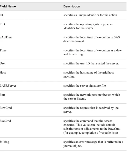
The following file content shows an example of three log records. Line breaks are added for readability. Each record is written on a single line and fields are separated by commas. Each field is a name-value pair.

(31)

File 1.1 Sample Log File Records

ID=1,PID=28622,SASTime=1658782485.36,Time=Tue Jul 24 20:54:45 2012,User=sasdemo, Host=grid001,LASRServer=/tmp/LASR.924998214.28622.saslasr,Port=56925,

RawCmd=action=ClassLevels name=DEPT.GRP1.PRDSALE "NlsenCoding=62",

ExeCmd=action=ClassLevels name=DEPT.GRP1.PRDSALE "NlsenCoding=62",JnlMsg=, StatusMsg=Command successfully completed.,RunTime= 2.17

ID=2,PID=28622,SASTime=1658782593.09,Time=Tue Jul 24 20:56:33 2012,User=sasdemo, Host=grid001,LASRServer=/tmp/LASR.924998214.28622.saslasr,Port=56925,

RawCmd=action=BoxPlot name=DEPT.GRP1.PRDSALE,

ExeCmd=action=BoxPlot name=DEPT.GRP1.PRDSALE,JnlMsg=,

StatusMsg=Command successfully completed.,RunTime= 0.12

ID=3,PID=28622,SASTime=1658825361.76,Time=Wed Jul 25 08:49:21 2012,User=sasdemo, Host=grid001,LASRServer=/tmp/LASR.924998214.28622.saslasr,Port=56925,

RawCmd=action=APPEND_TABLE ,ExeCmd=action=APPEND_TABLE ,JnlMsg=, StatusMsg=Command successfully completed.,RunTime= 0.09

Table 1.1 Log Record Fields

Field Name Description

ID specifies a unique identifier for the action. PID specifies the operating system process

identifier for the server.

SASTime specifies the local time of execution in SAS datetime format.

Time specifies the local time of execution as a date and time string.

User specifies the user ID that started the server. Host specifies the host name of the grid host

machine.

LASRServer specifies the server signature file.

Port specifies the network port number on which the server listens.

RawCmd specifies the request that is received by the server.

ExeCmd specifies the command that the server executes. This value can include default substitutions or adjustments to the RawCmd (for example, completion of variable lists). JnlMsg specifies an error message that is buffered in a

journal object.

(32)

Field Name Description

StatusMsg specifies the status completion message. RunTime specifies the processing duration (in seconds).

The server uses a journal object to buffer messages that can be localized. The format for the JnlMsg value is n-m:text.

n

is an integer that specifies the message is the nth in the journal. m

is an integer that specifies the message severity. text

is a text string that specifies the error.

Sample JnlMsg Values

JnlMsg=1-4:ERROR: The variable c1 in table WORK.EMPTY must be numeric for this analysis.

JnlMsg=2-4:ERROR: You do not have sufficient authorization to add tables to this LASR Analytic Server.

Data Compression

Overview of Data Compression

SAS LASR Analytic Server supports compression for in-memory tables. All the analytic statements, such as PERCENTILES, LOGISTIC, and so on, in the IMSTAT procedure are supported for compressed tables as well as regular, uncompressed, tables. Clients like SAS Visual Analytics can also operate on compressed tables as well.

All compression is performed by the server. In other words, when you transfer a table to the server in a DATA step and specify the SQUEEZE= data set option, the rows are sent to the server as is, and the server compresses the rows. The server uses the zlib

compression algorithm that is described in RFC 1950, "ZLIB Compressed Data Format Specification."

All data in a row, both character and number variables, are compressed. Every row in a table is compressed, the server does not support some rows in compressed form and others as uncompressed. The server can report the uncompressed size of the table, the compressed size, and the compression ratio.

For matrices of computed doubles (with lots of decimal places), compression might not reduce the storage requirements at all. For rows with many long character variables that consist mostly of blanks, the compression ratio can be very high. For rows with mixed variables where most doubles do not have fractional parts and most character variables have a small amount of blank padding, the compression ratio is typically moderate. As with most cases of using compression, character variables tend to compress the most and the ratio depends on your data.

(33)

Compressed Tables and the DATA Step

The following example shows how to use the SQUEEZE= data set option for the SAS LASR Analytic Server.

Example Code 1.1 Creating a Compressed Table with a DATA Step

libname example sasiola host="grid001.example.com" port=10010 tag=hps; data example.prdsale(squeeze=yes);

set sashelp.prdsale; run;

After the table is loaded to memory, you can access the compressed table with the Example.Prdsale libref.

The server supports the APPEND= option for compressed tables. The following example shows how to add new rows (uncompressed) to the compressed table:

Example Code 1.2 Appending Rows to a Compressed Table data example.prdsale(append=yes);

somelib.newrows; run;

Because the Example.Prdsale table is already compressed, the new rows are

automatically compressed as they are appended to the table. Specifying SQUEEZE= with APPEND= has no effect. If the table is compressed, the server compresses the new rows. If the table is not compressed, the server does not compress the new rows (even if SQUEEZE=YES is specified). The compressed or uncompressed state of the table determines how the rows are appended.

Partitioning and compression are supported together. The following example creates a new in-memory table that is partitioned and compressed:

Example Code 1.3 Creating a Partitioned and Compressed Table data example.iris(partition=(species) squeeze=yes); set sashelp.iris;

run;

data example.iris(append=yes); set somelib.moreirises; run;

In the first DATA statement, the Iris data set is loaded to memory on the server and is partitioned by the formatted values of the Species variable. The table is also compressed. In the second DATA statement, the table is appended to with more rows. Because the in-memory table is already partitioned and compressed, the new rows are automatically partitioned and compressed when they are appended.

Compressed Tables and the LASR Procedure

The LASR procedure is used for loading data to memory on distributed SAS LASR Analytic Server.

The following example shows how to read a SAS data set and compress it in memory on the server:

proc lasr add data=sashelp.prdsale port=10010 squeeze;

(34)

performance host="grid001.example.com"; run;

The example uses the SQUEEZE option to read the Prdsale data set from the Sashelp library and compress it in-memory on the server. Be aware that you must specify the SQUEEZE option for each table that you want to load in compressed form. You cannot specify SQUEEZE with the CREATE option when you start a server and have the server automatically compress all tables.

The SQUEEZE option works when reading data from SAS/ACCESS engines, too. The resulting in-memory table is compressed whether you read data serially from a standard database or you read data in parallel from a distributed database like Greenplum Database.

When you read SASHDAT tables into memory, the compression for the resulting in-memory tables depends on the following:

• whether a WHERE clause is used

• whether the SASHDAT table is compressed on disk

If you specify a WHERE clause and the SQUEEZE option, then the server evaluates the WHERE clause as it reads data from HDFS and compresses the rows that meet the WHERE clause criteria. The memory efficiencies of the SASHDAT table format are forfeited in this scenario because the server had to apply the WHERE clause.

If you do not specify a WHERE clause, then the server ignores the SQUEEZE option and relies on whether the SASHDAT table is compressed. If the SASHDAT table is compressed, then the in-memory representation of the table is also compressed. If the SASHDAT table is not compressed, then the in-memory representation is not compressed either. The server ignores the option so that it can keep the memory efficiencies of the SASHDAT table format—when a SASHDAT table is loaded to memory, the in-memory representation is identical to the on-disk representation. Performance Considerations

Compression exchanges less memory use for more CPU use. It slows down any request that processes the data. An in-memory table consists of blocks of rows. When the server works with a compressed table, the blocks of rows must be uncompressed before the server can work with the variables. In some cases, a request can require five times longer to run with a compressed table rather than an uncompressed table.

For example, if you want to summarize two variables in a table that has 100 variables, all 100 columns must be uncompressed in order to locate the data for the two variables of interest. If you specify a WHERE clause, then the server must uncompress the data before the WHERE clause can be applied. Like the example where only two of 100 variables are used, if the WHERE clause is very restrictive, then there is a substantial performance penalty to filter out most of the rows.

Working with SASHDAT tables that are loaded from HDFS is the most memory-efficient way to use the server. Using compressed SASHDAT tables preserves the memory efficiencies, but still incurs the performance penalty of uncompressing the rows as the server operates on each row..

Interactions

The interactions for compressed tables and SAS programs are as follows: • You can use a compressed table in programs like any other table.

(35)

• You can define calculated columns for compressed tables with the COMPUTE statement or with the TEMPNAMES= and TEMPEXPRESS= options.

• You can use SIGNER= security with compressed tables.

• You can append to compressed tables with the SET statement or the APPEND= data set option. This is also supported for compressed tables that have partitioning. However, you cannot append to a compressed table that is partitioned and has an ORDERBY specification.

• You can use the UPDATE statement with a compressed table.

• You can use a compressed table with a statement in the IMSTAT procedure that produces a temporary table. Whether the resulting temporary table is compressed depends on whether you specify the TEMPSQUEEZE option in the IMSTAT procedure. The following statements in the IMSTAT procedure support creating temporary tables:

• ACCESS

• AGGREGATE

• BALANCE • CLUSTER • CROSSTAB • DECISIONTREE • DISTINCT • GENMODEL

• GLM

• GROUPBY

• LOGISTIC

• MDSUMMARY

• PARTITION • PERCENTILE

• RANDOMWOODS

• SCHEMA (does not support creating compressed temporary tables) • SCORE

• SUMMARY

• You can use the BALANCE and PARTITION statements to create a compressed table when the TEMPSQUEEZE option is used. Applying orderby and compression at the same time has a significant performance penalty.

• You can use the UNCOMPRESS statement with a compressed and partitioned table. The temporary table that is created is partitioned according to the original table. • You can use DELETEROWS and the PURGE option with a compressed table. There

is a significant performance penalty for the PURGE option.

• You can create an empty table in compressed form, using either a DATA step or the CREATETABLE statement of the IMSTAT procedure. Although the table has no rows, rows that are appended to it later are compressed.

• You can use the SCORE statement with a compressed table.