Vol 63, No 1 (2020)

TECHNICAL UNIVERSITY OF CLUJ-NAPOCA

ACTA TECHNICA NAPOCENSIS

Series: Applied Mathematics, Mechanics, and Engineering Vol. 63, Issue I, March, 2020

FINITE ELEMENT USED IN THE DYNAMIC ANALYSIS OF A

MECHANICAL PLANE MBS WITH A PLANAR “RIGID MOTION”

Maria Luminita SCUTARU, Eliza CHIRCAN, Sorin VLASE, Marin MARIN

Abstract: The paper aims to study a finite element in the case of plane motion of a plane mechanical system.

The problem of using two-dimensional finite elements in the dynamic analysis of membranes has been little studied in the literature, which is mainly due to the formalism involved, which requires a special calculation effort. The evolution equations are established and the matrix coefficients are calculated. An example of calculating the eigenvalues for a rectangular shell is presented, which uses the formalism developed in the paper.

Key words: Multibody System (MBS), Finite Element Method (FEM), eigenfrequencies, eigenvectors,

shell, two-dimensional

1. INTRODUCTION

The last decades have been characterized by the development of multi-body systems (MBS) with deformable elements mostly in industrial applications. The first researches in the field were made for one-dimensional finite elements using third and fifth degree polynomial shape functions. Then the interest moved on to more complex, two-dimensional or three-dimensional finite elements.

The most common method to obtain the dynamic response of such a system is represented by Lagrange's equations [8-13]. Determining the evolution equations of a single element is the most important step in an analysis of an MBS system. The other procedures that follow in such an analysis are the classic ones, well known from the finite element commercial software. After all these steps, the evolution equations for this problem are obtained. The final shape of the matrix coefficients will ultimately depend on the interpolation functions chosen, for each individual case, for the finite

element used. In the present work we aim to determine the evolution equations of an element, used in the study of plane mechanisms with elastic elements[6],[7],[14],[15].

2. EQUATION OF MOTIONS

Consider the plate used for stress analysis in plane elasticity. Let us consider a single finite element referred to the local Oxy coordinate system, in solidarity with the finite element. This reference system is mobile and participates in the parallel plane motion of the plate. It is noted with v _{( , )} the speed and a _{( , )}

acceleration of the origin of the mobile reference system in relation to the fixed reference system O'XY. The mobile reference system will have angular velocity = and angular acceleration

[ ]

_   − = θ θ θ θ c s s c

R (1)

where is denoted c_θ =cosθ,s_θ =sinθ , makes

the transformation from the local to the global reference frame. A vector v(vx,vy) expressed in

the mobile reference system becomes, in the global reference system [3],[4]:

          − =       y x Y X v v c s s c v v θ θ θ

θ _{. (2)}

Fig.1. A rectangular finite element

{ }

rM G is the position vector of point M:

{ } { } { } { }

rM G = rO G + r G = rO G +

[ ]

R

{ }

r L (3) where the index G expresses a size in the fix reference frame and the index L shows that the size is written in the mobile reference frame. If M becomes M', undergoing a small displacement

{ }

f _L, one can write:

{ } { }

r_M' _G = r_{O G} +

[ ]

R

(

{ } { }

r _L + f _L

)

=

[ ]

            +       +      

= R x_y u_v

Y X

0

0 ₍₄₎

The continuous field of displacements is approximated, in the method of the finite elements, by the relation:

{ }

L _v

[

x y

]

{ }

t L

u

f = Φ( , ) δ()

     

= (5)

where

[

Φ

(x,y)

]

is the matrix of the shape function. The vector

{ }

δ(t) _L represents the vector of the independent coordinates, expressed in the mobile coordinate frame. We consider the displacements u and v of some point as completely defined by the nodal displacements. For this triangular finite element, with the nodes at the ends, the shape functions are chosen:

=               =       4 3 2 1 4 3 2 1 4 3 2 1 0 0 0 0 0 0 0 0 δ δ δδ Φ Φ Φ

Φ Φ Φ Φ

Φ

v u

[ ]

Φ

{ }

δ L

= (6)

{ }

_    = i i i _v u

δ , i=1,2 (7)

where it was noted:

b y a x = =

η

ξ

; ; (8)

(

1

)(

1

)

; ₂

(

1

)

;

1

ξ

η

Φ

ξ

η

Φ

= − − = −

(

ξ

)

η Φ ξη

Φ3 = ; 4 = 1− (9)

The velocity of point M 'can be expressed by:

′ = ′ = + +

+ ! "#+ ! !$"%_# (10)

The expression of kinetic energy for a single finite element is:





=

=

V V

c v dV

E

ρ

ρ

2 1 2

1 2

{ } { }

_{v v dV} G M T G

M' ' =

$"%_#, !, _!, _{! !$"%}

#++2   +

2   ! !$"%_#++2 0  0 !"/+

2 " /0 !0 0 ++2$"%# ,

!, _!, ₊

+2 " #, !, , ! !$"%_#)12 (11)

The concentrated and distributed loads gives us the work:

+ =



{ } { }

+

{ } { }

T _L=

V T

c _{p f dV q}

W

W

δ

(

{ }

[ ]

)

{ } { } { }

_L T _L V

T

q dV

p

Φ

δ

+

δ

=

_

(12)

The Lagrangian for the finite element considered is:

L=Ec−Ep+W+Wc . (13)

and the evolution equations were obtained with Lagrange method [14].

If you consider that:

a) _{( !*} , !, )314=

[ ] [ ]

[

]

 =            −      − =

_

V T T _tdA y x x y

FΦ ε ω ρ

Φ 2 ) 2 ( ) 1 (

[ ] [ ]

(

)

[ ] [ ]

(

+

)

= − − + − =





V T T V T T tdA y x tdA x y ρ Φ Φ ω ρ Φ Φ ε ) 2 ( ) 1 ( 2 ) 2 ( ) 1 (

{ }

{ }

(

my mx

)

(

{ }

m1x

{ }

m2y

)

2

2

1 + − +

−

=

ε

ω

(14)

It was noted:

{ }

=



V T

x x tdA

m₁ Φ₍₁₎ ρ ;

{ }

=



V

T

y y tdA

m₁ Φ₍₁₎ ρ ; (15)

{ }

=



V T

x x tdA

m₂ Φ₍₂₎ ρ ;

{ }

=



V

T

y y tdA

m₂ Φ₍₂₎ ρ . (16) b) ( !, _!, _!)314

* =

[ ]

[

]

_{[ ]}

[ ]



−       − = V T

T

_ρ

_tdA

Φ

Φ

Φ

Φ

ε

) 2 ( ) 1 ( ) 2 (

[ ] [ ]

[

]

_{[ ]}

[ ]

=       −

_

V T

T

_ρ

_tdA

Φ

Φ

Φ

Φ

ω

) 2 ( ) 1 ( ) 2 ( ) 1 ( 2

[ ] [ ] [ ] [ ]

(

)



− − = V T

T_{Φ Φ Φ ρtdA}

Φ

ε (2) (1) (1) (2)

[ ] [ ] [ ] [ ]

(

+

)

= −

_

V T T

T_{Φ Φ Φ ρtdA}

Φ

ω (1) (1) (2) (2) 2

[ ]

c _ω2

[ ]

m

ε −

= (17)

It was noted:

[ ]

=



(

[ ] [ ] [ ] [ ]

−

)

V

T

T _tdA

c Φ₍₂₎ Φ₍₁₎ Φ₍₁₎ Φ₍₂₎ ρ ;

[ ]

=



(

[ ] [ ] [ ] [ ]

+

)

V

T T

T _tdA

m Φ₍₁₎ Φ₍₁₎ Φ₍₂₎ Φ₍₂₎ ρ (18)

c)



[ ] [ ]

= V T tdA ρ Φ Φ

[ ] [ ] [ ] [ ]

(

+

)

= =

_

V T T

T_{Φ Φ Φ ρtdA}

Φ(1) (1) (2) (2)

[ ] [ ] [ ]

m + m = m

= 11 22 (19)

where it was noted:

[ ]

=



V j T i ij tdA

m Φ₍₎Φ_{( )}ρ (20)

d) _{( !}, _!, _!)314

* =

[ ] [ ]

[

]

_{[ ]}

[ ]

tdA

[ ]

c V

T

T

_ρ

_ω

Φ

Φ

Φ

Φ

ω

=       − =

_

) 2 ( ) 1 ( ) 1 ( ) 2 ( (21) It is also noted:



=

V

tdA

m ρ ;

[ ]

m

[ ]

T tdA ;

V i

o =



Φ ρ

{ }

_mi ₌

{ }

_{m1x +}

{ }

_m2y ;

ω

{ }

{ }

y

{ }

x

i _{m m}

56 7 (&) , (&) + (') , ('),8 )314

* 9 $"%#+

+2 56 7 ('), (&) − (&) , (')8 )314

* 9 $"%#+

+[

[ ]

(

[ ] [ ] [ ] [ ]

)

_−

  

  

−

+

_

V

T

T _tdA

k ε Φ(2) Φ(1) Φ(1) Φ(2) ρ

[ ] [ ] [ ] [ ]

(

)



  

  

+

−

_

V

T T

T_{Φ Φ Φ ρtdA}

Φ

ω (1) (1) (2) (2) 2

]

{ }

δ _L =

{ }

+

[ ]

{ }

−

=

_

V T

L p tdA

q Φ ρ

− 56 (&), ('), )314

* 9 ! −

[ ] [ ]

[

−

+

]

+

−

_

V

T

T

_y

_Φ

_x

_ρ

_tdA

Φ

ε

(1) (2)

[ ] [ ]

[

]



+

+

V

T T_{x Φ y ρtdA}

Φ

ω (1) (2) 2

(23) or:

( ;&&! + ;''!)$"%_#+ 2 ( ;'&! − ;&'!)$"%_#+

[ ] [ ] [ ]

(

)

(

[ ] [ ]

)

[

+ − − +

]

{ }

= + ke

ε

m m

ω

m11 m22

δ

L

2 12 21

= < #+ <∗ #− ;!(&), ;!('), > ? −

[ ]

[ ]

(

)

(

[ ] [ ]

T

)

y T x x

y m m m

m 2 _{1 2}

2

1 + + +

−

−ε ω (24)

or:

;!$"%_#+ @!$"%_#+ AB! + @!−⥂ ';! " =

= < #+ <∗ #− ;D! > ? − ;ED + ' ;FD

(25) Now it is possible to determine the matrix coefficients accordingly.

3. EXAMPLE

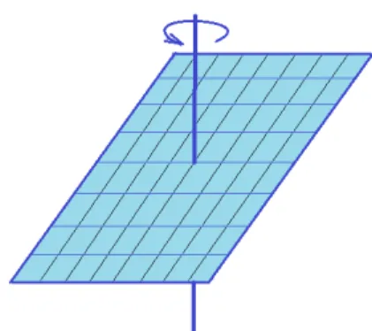
Consider a plate with the dimension length = 0.2 m and width = 0.16 m. The thickness = 0.001 m and the Young’s modulus = 210 GPa. The mass density is 7800 kg/m3 _(Fig.2).

Fig. 2. Rectangular plane plate in rotation

Using FEA, meshing the plate and written the motion eqautions for the entire shell is possible to obtain eigenvalues. In Fig.3 we present the first 15 eigenvalues. The angular speed is varied between 5,000 and 15.000 rad/s.

Fig.3. First 15 eigenvalues for different angular speed

Fig.4. First 15 eigenvalues for angular speed 14,000 rad/s

4. CONCLUSIONS

In the paper are obtained the evolution equations for a rectangular element used for the study of multi-body mechanical systems with elastic elements. Lagrange method were used to obtain these. Specific shape functions were used for this type of finite element, known from the static or steady state analysis. It is presented, for example, the calculation for a plate in rotation. The main problem for such an analysis is the volume of calculation required to obtain the matrix coefficients of the equations of motion.

5. REFERENCES

[1] Itu, C., Ochsner, A., Vlase, S., Marin,M.,

Improved rigidity of composite circular plates through radial ribs. Proceedings of the Institution of Mechanical Engineering-Design and Applications. Vol.233, Issue 8 (2019) pp.1585-1593.

[2] Katouzian,M., Vlase, S., Calin, M.R.,

Experimental procedures to determine the viscoelastic parameters of laminated composites. Journal of Optoelectronic and Advanced Materials. Vol.13, Issue 9-10 (2011) pp.1185-1188.

[3] Jurco, SG, Jurco, E., Tomoaia, Gh., Arghir, M., Study of Human Body Mobility through Mechanical Modeling. Acta Technica Napocensis, Series: Applied Mathematics, Mechanics and

Engineering, Vol 60, No 1 , 137-142, 2017.

[4] Jurco,SG, Jurco, EC, Tomoaia, Gh, Arghir, M., Onaciu, Gr., Mechanical Modeling 4-EPPC Corresponding to Legs, Pelvis and Body, Supported on a Rigid Support with One Leg on Excitation. Acta Technica Napocensis, Series: Applied Mathematics, Mechanics and Engineering, Vol 61, No 1, pp.17-22, 2018.

[5] Massonet, Ch. Et al, Calcul des structures sur ordinateur. Eyroll EDITEUR, 1972 [6] Marin, M., Chirila, A., Ochsner, A., Vlase,

S , About finite energy solutions in thermoelasticity of micropolar bodies with voids. Boundary Value Problems, Article Number: 89, DOI: 10.1186/s13661-019-1203-3, 2019.

[7] Marin,M., Agarwal, R.P., Mahmoud,S.R.,

Nonsimple material problems addressed by the Lagrange's identity, Boundary Value Problems, vol. 2013, 1-14, 2013, Art. No. 135.

[8] Negrean I., New Formulations in Analytical Dynamics of Systems, published in Acta Technica Napocensis, Series: Applied Mathematics, Mechanics and Engineering, Vol. 60, Issue I, ISSN 1221-5872, pp. 49-56, 2017.

[9] Negrean I., Advanced Notions in Analytical Dynamics of Systems, published in Acta Technica Napocensis, Series: Applied Mathematics, Mechanics and Engineering, Vol. 60, Issue IV, ISSN 1221-5872, pp. 491-502, 2017.

[10] Negrean I., New Approaches on Notions from Advanced Mechanics, published in Acta Technica Napocensis, Series: Applied Mathematics, Mechanics and Engineering, Vol. 61, Issue II, ISSN 1221-5872, pp. 149-158,2018.

[11] Negrean I., Formulations on Input Parameters in Advanced Dynamics, published in Acta Technica Napocensis, Series: Applied Mathematics, Mechanics and Engineering, Vol. 61, Issue III, ISSN 1221-5872, pp. 305-312, 2018.

[12] Negrean, I., Crișan, A.-D. Synthesis on the

Acceleration Energies in the Advanced

5,5 6 6,5 7 7,5

1 2 3 4 5 6 7 8 9 101112131415

E

ig

e

n

v

a

lu

e

s/

1

0

e

5

[H

z/

1

0

e

5

]

Mechanics of the Multibody Systems. Symmetry,2019, 11(9), 1077.

[13] Negrean, I., Crișan, A.-D., Vlase, S. A New

Approach in Analytical Dynamics of

Mechanical Systems. Symmetry,

2020,12(1), 95.

[14] Vlase, S., Dynamical Response of a Multibody System with Flexible Elements with a General Three-Dimensional Motion. Romanian Journal of Physics, Vol. 57, Issue 3-4, pp. 676-693, 2012. [15] Vlase, S., Marin, M., Öchsner, A., Scutaru,

M.L. Motion equation for a flexible

one-dimensional element used in the dynamical analysis of a multibody system. Continuum Mech. Thermodyn., 2019, doi.org/10.1007/ s00161-018-0722-y. [16] Vlase, S., Danasel, C., Scutaru, M. L.,

Mihalcica, M., Finite Element Analysis of a Two-Dimensional Linear Elastic Systems with a Plane "Rigid Motion".

Romanian Journal of Physics, Vol.59, Issue 5-6, pp.476-487, 2014.

Element finit dreptunghiular în stare de membrană pentru analiza dinamică a unui sistem multicorp cu o mișcare plană

Rezumat Lucrarea își propune dezvoltarea unui element finit dreptunghiular pentru studiul

mișcărilor plane ale unei plăci în stare de membrană. Problema utilizării elementelor finite

bidimensionale în analiza dinamică a membranelor este puțin aboordată în literatură, lucru datorat

mai ales formalismului implicat, care necesită un efor de calcul deosebit. În lucrare sunt stabilite

ecuațiile de mișcare pentru elementul finit studiat și sunt calculați coeficienții matriceali. Un exemplu

de calcul al valorilor proprii pentru o placă dreptunghiulară este prezentat, care utilizează

formalismul dezvoltat în lucrare.

Maria Luminița SCUTARU, Professor, Dr. hab., Transylvania University of Brașov, Department

of Mechanical Engineering, [email protected], Office phone: +40-268-418992, 29, B-dul Eroilor, 500036, Brașov, home phone: +40-723-242735.

Eliza CHIRCAN, Ph.D. student, Transylvania University of Brașov, Department of Mechanical

Engineering, [email protected], Office phone: +40-268-418992, 29, B-dul Eroilor, 500036, Brașov.

Sorin VLASE, Prof.Dr.hab.,Head of Department, Transylvania University of Brașov, Department

of Mechanical Engineering, [email protected], Office phone: +40-268-418992, 30, Castelului, 500014, Brașov, home phone: +40-722-643020.

Marin MARIN, Prof. Dr.hab., Transylvania University of Brașov, Department of Mathematics,