Copyright © 2017 Vilnius Gediminas Technical University (VGTU) Press Technika http://www.bjrbe.vgtu.lt
doi:10.3846/bjrbe.2017.31 OF ROAD AND BRIDGE ENGINEERING
ISSN 1822-427X / eISSN 1822-4288 2017 Volume 12(4): 248–257
1. Introduction
Due to large span ability and wind resistance stability, ca-ble-stayed bridges have become popular in recent years, consisting of the tower, girder, cable and other compo-nents. Besides the dead load, wind load, seismic load, and temperature load, the vehicle load is acritical load that is taken into account in the design of cable-stayed bridges. The vehicle load resulting from the traffic flow on the bridge is a stochastic process, varying with time and location. In cur-rent main design codes, for instance, Load and Resistance Factor Design (LRFD) Bridge Design Specifications, Ameri-can Association of State Highway and Transportation Of-ficials (AASHTO:2014); JTG D60-2015 General Code for Design of Highway Bridges and Culverts, Ministry of Com-munications, Beijing, China; CEN 2003. Eurocode 1: Actions on Structures − Part 2: Traffic Loads on Bridges, Brussels, the vehicle load is treated as a notional static load that is inca-pable of accurate representation of actual vehicle weights. For short and medium span bridges, the load effects (i.e., the moment and shear) using the superposition of vehicle and lane load within a single design lane that represent the actual load effects accurately. However, this method has
limitations for long-span bridges, on which there is simul-taneous presence of multiple vehicles. Some recent studies adopted an assumed (usually uniform) pattern of several ve-hicles distributed on a long-span bridge in considering the vehicle load(Calcada et al. 2005; Chen et al. 2006; Zhou, Chen 2015). In fact, this assumption obviously differs from reality, in which vehicles move randomly through a bridge following traffic rules. It is essential to take into account the random vehicle load when analysing the load effects of long-span bridges. Moreover, Articles 44 and 78 of the Regulation on the Implementation of the Road Traffic Safety Law of the People’s Republic of China by State Council, Beijing, China of 2003 stipulate that the expressway has two or more traf-fic lanes in the same direction. The left side lane is the fast lane, the right side lane is the slow lane. Thus, the probability model of vehicle load in the fast lane (left lane), middle lane and slow lane (right lane) are respectively established based on actual traffic flow.
Nowadays, vehicle load data are usually collected through Weight-in-Motion (WIM) or traffic spectrum from the site (Mullard, Stewart 2009; Oh et al. 2007). However, neither of these methods provides instantaneous velocity
PROBABILITY MODEL AND RELIABILITY ANALYSIS OF CABLE STRESS
FOR CABLE-STAYED BRIDGE
Xiao-Yan Yang1, Jin-Xin Gong2, Yin-Hui Wang3, Bo-Han Xu4, Ji-Chao Zhu5
1, 3School of Civil Engineering & Architecture, Ningbo Institute of Technology, Zhejiang Univ., Ningbo 315100, People’s Republic of China
1, 2, 4State Key Laboratory of Coastal and Offshore Engineering, Dalian University of Technology, Linggong Road, Ganjingzi District, Dalian 116024, People’s Republic of China
5School of Civil Safety Engineering, Dalian Jiaotong Univ. of Technology, Dalian 116028, People’s Republic of China E-mails: 1[email protected]; 2[email protected]; 3[email protected];
4[email protected]; 5[email protected]
Abstract: The aim of this paper is to investigate the time-varying effect of stay cable of long-span cable-stayed bridges subject to vehicle load. The analysis has been carried out on the Su-Tong cable-stayed bridge in Jiangsu, China that has the second-longest span among the completed composite-deck cable-stayed bridges in the world currently. Probability models of vehicle load in each lane (fast lane, middle lane and slow lane) and cable stress under random vehicle load were developed based on the stochastic process theory. The results show the gross vehicle weight follows lognormal distribution or multi-peak distribution, and the time-interval of the vehicle follows a lognormal distribution. Then, the probability function of maximum cable stress was determined using up-crossing theory. Finally, the reliability of stay cable under random vehicle load was analysed. The reliability index ranges from 9.59 to 10.82 that satisfies the target reliability index of highway bridge structure of finished dead state.
and position information of the individual vehicle, it is es-sential to the assessment of time-varying loads for long-span bridges. There are also several simple random pro-cesses for the traffic flow simulation such as white noise fields (Ditlevsen 1994; OBrien et al. 2015) and Poisson dis-tribution (Sun 2015). Nevertheless, they are challenging to address relatively complicated vehicle load in long-span bridges. Monte-Carlo approach is a practical and straight-forward method, which is used to generate traffic data fol-lowing the existing or assumed statistical distribution of the traffic flow (Moses 2001; O’Connor, O’Brien 2005).
This study used statistical analysis of cable stress of Su-Tong cable-stayed bridge based on the vehicle load from la-test survey traffic flow data, and developed the probability models of random vehicle load and maximum cable stress in design reference period. Also, reliability analysis of the stay cable under random vehicle load was also accomplished. 2. Cable stress calculation
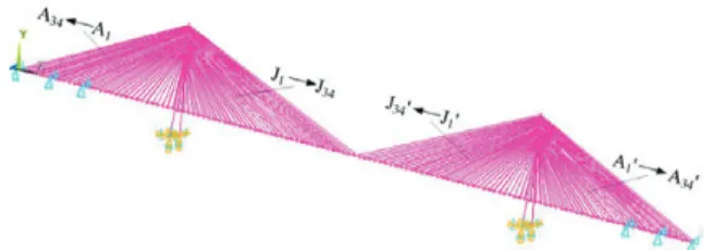
The cable stress of Sutong Yangtze River Bridge was cal-culated by the vehicles moving and time-varying status. Su-Tong cable-stayed bridge (Fig. 1) connects Suzhou and Nantong of Jiangsu province and is the second-longest ca-ble-stayed bridge in the world with a main span of 1088 m (Xi et al. 2014). This sea-crossing bridge is a double-tow-er and double-cable-plane steel-box girddouble-tow-er cable-stayed bridge that was opened to traffic on 25th May 2008. Its design reference period is 100 years. The streamlined flat steel-box girder is employed in the bridge. The overall width of the girder is 34.0 m consisting of two-way six 3.75 m lanes, two 3.50 m emergency lanes, and two 2.25 m shoul-ders. Parallel wire cables are adopted with intervals being 16 m on the deck and 2 m on the towers. The total number of cables is 272 (4×34×2). Design working life of the stay cable is 50 years. Among them, the longest cable is 577 m that is record-breaking. The two main towers are inverted Y-shaped. The overall height of the towers is 300.40 m, mak-ing them the tallest bridge towers in the world.
The three-dimensional finite element analysis (FEA) model developed in this study is shown in Fig. 1. Both girder and tower are modelled using beam elements (BEAM44) with six degrees of freedom at each node. The cables are modeled as link elements (LINK10) with initial tension stress. The non-linear behaviour of cables due to their sags is taken into account by using an equivalent mo-dulus of elasticity (Wang et al. 2013). Regarding the boun-dary conditions, the girder is free to move in the longitudi-nal direction and restrained at the supports in the vertical and transverse directions. Only the rotational component around the longitudinal axis is restrained. The tower bases are fixed in all degrees of freedom. In this model, auxiliary girder is adopted to resist the horizontal load action, and the larger elastic modulus is adopted to improve the lateral stiffness of main girder (Zhang et al. 2001). The material properties of the bridge are shown in Table 1.
2.2. Cable stress of dead load
Dead load of cable-stayed bridge G consists of the first dead load and second dead load. The first dead load includes the
weights of girder, tower, and cable. The weights of girder and tower are based on the actual cross-section properties. The weight of cable is obtained according to the required weight of steel. The second dead load is calculated according to the uniformly distributed load of 62.5 kN/m (Zhang, Chen 2010). The dead load of the cable-stayed bridge is calculat-ed by ANSYS program. Because of the small variability, the dead load of long-span cable-stayed bridges slightly fluctu-ates around its average value. In the meantime, cable stress is considered as linearly proportional to load. Thus, the mean value of cable stress is obtained by the mean value of the dead load, and the coefficient of variation remains constant. GB/T 50283–1999 Unified Standard for Reliability Design of Highway Engineering Structures, Highway Planning and De-sign Institute of the Ministry of Transport, Beijing, China specified that the bias coefficient (the ratio of mean value to nominal value) of dead load is 1.0148, the coefficient of vari-ation is 0.0431, and the probability distribution of dead load follows normal distribution JTG D60-2004. The mean stress values of cable No. A13–A18 produced by a dead load of the bridge (µG) are shown in Table 2.
Fig. 1. Finite element analysis model of Sutong highway bridge
Table 1. Material mechanical properties
Material property
Main
girder Auxiliary girder towerMain cableStay Steel Steel Concrete steel wireParallel Elasticity
modulus,
N/m2 2.10·1011 3.50·1013 3.25·1010 1.95·1011
Shear modulus,
N/m2 8.10·1010 8.10·1012 1.42·1010 –
Density,
kg/m3 7 900 7 900 2 600 7 900
Poisson
ratio 0.30 0.30 0.20 0.25
Table 2. Statistical parameters of cable stress under dead load of bridge and random vehicle load
Cable No. µG, MPa µX, MPa σX, MPa
A13 126.19 15.68 3.47
A14 128.55 16.19 3.72
A15 129.46 18.69 4.07
A16 129.35 20.69 4.29
A17 128.78 23.75 4.63
2.3. Cable stress of random vehicle load
The bridge load model is very closely related to gross ve-hicle weight, axle load, and inter-veve-hicle spacing. Also, the number and position of wheels change with time as the vehicle moves on a bridge (Helmi et al. 2014, Xu et al. 2015). In other words, the gross vehicle weight, axle load, and inter-vehicle spacing are all the random variables. Thus, the cable stress under vehicle load is a stochastic process. Weighing vehicles, which travel on highways, are known as WIM technology. By using a WIM system, vir-tually a 100% sample of traffic data for statistical purposes is obtained. The information is transmitted immediately in real time, or at a future time, to locations remote from the WIM site via conventional communications networks (Miao, Chan 2002). Thus, WIM systems were used to pro-vide a significant amount of traffic flow data. These data were then used to determine the mathematical distribu-tions and statistical parameters of the bridge random ve-hicle load.
For long-span cable-stayed bridges, vehicle load occu-pies a small proportion of vertical load (10–20%). Thus, the total cable stress is obtained by superposition of cable stress induced by vehicle load and produced by a dead load of the bridge. Through the supposition of cable stress obtained
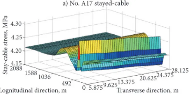
from influence surface for various vehicle positions, the ca-ble stress under vehicle load in multi-lanes is obtained. 2.3.1. Influence surface of cable stress
Besides dead load of bridge (mean value was adopted), the standard axle load of 100 kN (CJJ 37-2012 Code for De-sign of Urban Road Engineering, Ministry of Housing and Urban-Rural Development, Beijing, China) as the unit force was successively applied on node of deck element, in which the wheel arrives. According to the principle of superposition, cable stress of vehicle load is obtained by subtracting the cable stress produced by the dead load of the total cable stress. Thus, the influence surface of each cable stress as vehicle moves on the deck of the bridge is es-tablished. Figure 2 shows the influence surface of No. A17 and No. A34 cable stress with unit force.
2.3.2. Random vehicle load from Weight-in-Motion data The maximum likelihood estimation approach is adopted to fit traffic flow data recorded by WIM systems. Then, the obtained statistical parameters such as mean value and standard deviation are verified by Kolmogorov-Smirnov (K-S) test method (Miao, Chan 2002). WIM system was used to record actual traffic situations having some limita-tions, while Monte-Carlo simulation was used to regener-ate traffic records for any chosen scenario.
1. Proportions of different types of vehicles
The proportions of different types of vehicles in the fast lane (left lane), middle lane and slow lane (right lane) are obtained by statistical analysis of the actual traffic flow, as shown in Table 3.
2. Gross vehicle weights
When statistical analysis is conducted for the proba-bility distribution of gross vehicle weight, the following underlying assumptions shall be made:
1) live load on the bridge only considers the action of the vehicle load, regardless of the influence of other factors;
2) the operating status of vehicle load in the fast lane, middle lane, and slow lane is considered, respec-tively. The stochastic process of vehicle load and a number of the vehicle are independent in each lane. The gross vehicle weights of two-axle cars obey the lognormal distribution, and Eq (1) gives the probability density function: 2 ln 1 ln 1 ln 1 ln( ) 1 1
( ) exp
2 2 G Gi G G g f g g
− µ
= −
σ
πσ , (1)
where µlnG1, σlnG1 − the mean and standard deviation of the logarithm of the ith two-axle car, respectively.
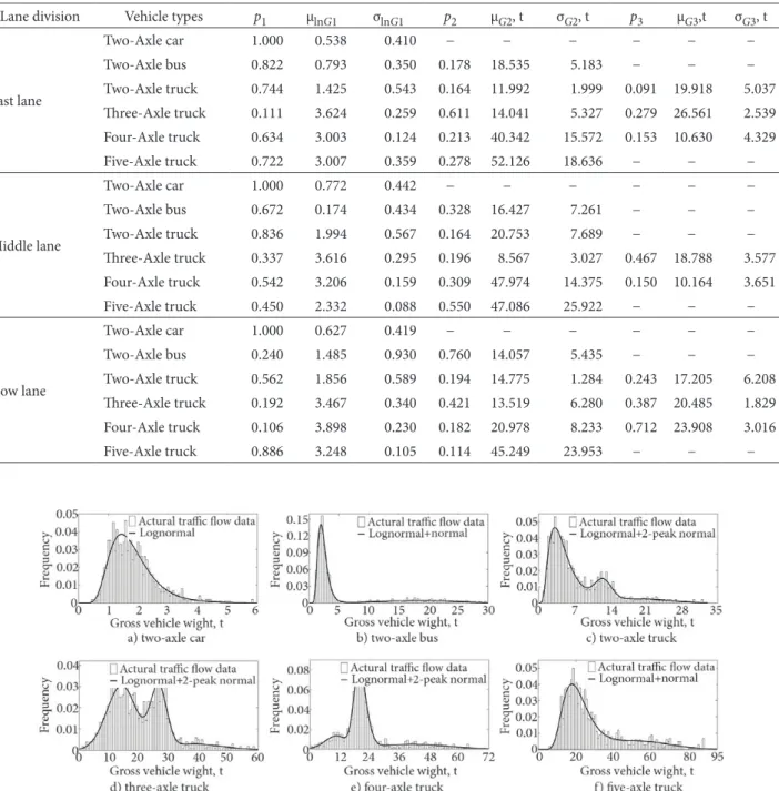
A multi-peak distribution with two or three peaks consists of a weighted sum of lognormal distribution and normal distributions, appropriately describing the gross vehicle weight of two-axle buses, two-, three-, four-, and five-axle trucks. The multi-peak probability density function is given by Eq (2):
Fig. 2. Influence surface of cable stress under unit load
Table 3. Proportions of different types of vehicles
Lane division
Percentage of vehicle types, %
Tw o-A xle Car s Tw o-A xle Bu se s Tw o-A xle Tr uc ks Thr ee-A xle Tr uc ks Fo ur -A xle Tr uc ks Fi ve-A xle Tr uc ks
ln 1 1
ln 1
ln( )
( ) G
G
Gi G
g p
f g g
− µ
= ϕ +
σ σ
2 1 1
n n
i Gi
i
Gi Gi
i i
p g
p
= =
− µ
ϕ =
σ σ
∑
∑
, (2)where µlnG1, σlnG1 – the mean and standard deviation of the lonarithm of the 1th overall vehicle load, respectively; µGi, σGi – the mean and standard deviation of the ith over-all vehicle load, respectively; p1 – the proportion of the 1st overall vehicle load; pi – the proportion of the ith overall vehicle load; ϕ(⋅) – the probability density function of the standard normal random variable.
These statistical parameters are summarized in Ta-ble 4. Figures 3–5 illustrate the statistical histograms of the gross vehicle weights of different types of vehicles and their fitted theoretical distributions.
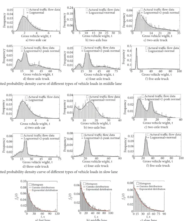
3. Time-interval of vehicle
The statistical analysis is also carried out to determine time-interval in vehicle load model. According to measured data of traffic flow, the histograms of the acquired data are shown in Fig. 6. Gamma distribution and exponential dis-tribution are to be merged for K-S test and confidence level α = 0.05 is adopted. The result shows that time-interval of the vehicle obeys gamma distribution and exponential distribution.
Table 4. Statistical parameters of gross vehicle weight
Lane division Vehicle types p1 µlnG1 σlnG1 p2 µG2, t σG2, t p3 µG3,t σG3, t
Fast lane
Two-Axle car 1.000 0.538 0.410 − − − − − −
Two-Axle bus 0.822 0.793 0.350 0.178 18.535 5.183 − − − Two-Axle truck 0.744 1.425 0.543 0.164 11.992 1.999 0.091 19.918 5.037 Three-Axle truck 0.111 3.624 0.259 0.611 14.041 5.327 0.279 26.561 2.539 Four-Axle truck 0.634 3.003 0.124 0.213 40.342 15.572 0.153 10.630 4.329 Five-Axle truck 0.722 3.007 0.359 0.278 52.126 18.636 − − −
Middle lane
Two-Axle car 1.000 0.772 0.442 − − − − − −
Two-Axle bus 0.672 0.174 0.434 0.328 16.427 7.261 − − − Two-Axle truck 0.836 1.994 0.567 0.164 20.753 7.689 − − − Three-Axle truck 0.337 3.616 0.295 0.196 8.567 3.027 0.467 18.788 3.577 Four-Axle truck 0.542 3.206 0.159 0.309 47.974 14.375 0.150 10.164 3.651 Five-Axle truck 0.450 2.332 0.088 0.550 47.086 25.922 − − −
Slow lane
Two-Axle car 1.000 0.627 0.419 − − − − − −
Two-Axle bus 0.240 1.485 0.930 0.760 14.057 5.435 − − − Two-Axle truck 0.562 1.856 0.589 0.194 14.775 1.284 0.243 17.205 6.208 Three-Axle truck 0.192 3.467 0.340 0.421 13.519 6.280 0.387 20.485 1.829 Four-Axle truck 0.106 3.898 0.230 0.182 20.978 8.233 0.712 23.908 3.016 Five-Axle truck 0.886 3.248 0.105 0.114 45.249 23.953 − − −
Probability density function of the gamma distribu-tion is as follows in Eq (3):
1
( ) ( )
a
a bt
T b
f t t e
a − −
=
Γ , (3)
where t – the random variable of time-interval of the ve-hicle, s; Γ(⋅) – gamma function; a and b – parameters.
Probability density function of exponential distribu-tion is as follows in Eq (4):
( ) t
T
f t = λe−λ , (4)
where λ − parameter.
For the statistical parameter of time-interval of the vehicle in Fig. 6a – a = 0.9670, b = 0.0449, λ = 0.0464; for data in Fig. 6b – a = 1.1231, b = 0.0603, λ = 0.0537; for data in Fig. 6c – a = 1.2402, b = 0.0604, λ = 0.0481. Fit-ted parameter a of time-interval of the vehicle with gam-ma distribution is close to 1. Time-interval of the vehicle approximately obeys exponential distribution to simplify the calculation.
4. Axle-weight proportion and axle spacing of different types of vehicle
The typical axle spacing of the different types vehicle were determined from 79 types of buses and 541 types of trucks presently available in China, as well as more than 200 thousand vehicles from traffic flow data. By regression Fig. 4. Fitted probability density curve of different types of vehicle loads in middle lane
Fig. 5. Fitted probability density curve of different types of vehicle loads in slow lane
analysis, the axle weight proportion and axle spacing of six types of representative vehicles mentioned above are sum-marized in Table 5.
2.3.3. Bridge loading
According to random vehicle load model in Section 2.3.2, six groups of random vehicle loads are generated through Monte-Carlo method, and the vehicle loads traveling in the two-way six lanes and then are placed in each lane. The traffic flow of random vehicle is generated through Monte-Carlo simulation as the flow chart shown in Fig. 7. The procedure used the site-specific vehicle characteristics of vehicle and axle weights. Only the cable stress of No. A1– A34 and No. J1–J34 were analysed considering geometri-cal symmetry.
3. Probability model of cable stress under vehicle load 3.1. Characteristics of cable stress
Stay cables are subject to loads varying with both time and space. For long-span cable-stayed bridges, the
Table 5. Axle weight proportion and axle spacing of different kinds of vehicles
Vehicle types
Proportion of axle weight Inter-axles distances, m
A
xle 1 Axle 2 Axle 3 Axle 4 Axle 5 xle 6A Axle 1-2 Axle 2-3 Axle 3-4 Axle 4-5 Axle 5-6
Two-Axle bus 0.26 0.74 − − − − 5.00 − − − −
Two-Axle truck 0.39 0.61 − − − − 3.00 − − − −
Three-Axle truck 0.15 0.44 0.41 − − − 5.00 1.30 − − −
Four-Axle truck 0.10 0.19 0.36 0.35 − − 2.50 6.00 1.30 − −
Five-Axle truck 0.06 0.27 0.24 0.22 0.22 − 3.40 7.40 1.30 1.30 − Six-Axle truck 0.04 0.19 0.17 0.21 0.19 0.21 3.20 1.50 7.00 1.30 1.30
Fig. 7. Flow chart of cable stress under random vehicle load
cable stress on different arbitrary-time point caused by the same vehicle is related. The stochastic process meth-od is adopted for each point. As the average speed of ve-hicle v was roughly 70 km/h (19.44 m/s), the duration of a continuous load applied to the structure is defined as
0.5 0.03 19.44 s t
v
∆
τ = ∆ = = = s, where Δs is distance-interval of 0.5 m, τ is a time interval. Hence, the cable stress caused by random vehicle load at the different arbitrary-time point is regarded as a sample function X(t) of a stochastic process. The mean value (µX) and standard deviation (σX) of sample function are given in Table 2.
The mean function and auto-correlation function of a stochastic process are used to describe the stochastic process. The auto-correlation function presents the corre-lation among any two adjacent times t1, t2 in a stochastic process, which are defined as (Eq (5)):
(
)
(
1 2)
1 2
1 2
, ,
( ) ( )
X X
X X
Cov t t t t
t t
ρ =
σ σ ,
(
1 2,)
{
( )1 ( )1 ( )2 ( ) ,2}
X X X
where ρX(t1, t2) – auto-correlation function; CovX(t1, t2) – covariance function; µX(t) – mean value of stochastic process X(t); σX(t) – standard deviation of a stochastic process X(t).
The white noise process is a sequence of independent, identically distributed random variables. If the influence sur-face was different from zero over a length, and it was longer compared to the length occupied by single vehicle, the white noise would be sufficient to model the load effects (stress, strain, bending) (Madsen 2007). However, as the influence surface was sufficiently slowly varying over steps continuity, and the ratio between the bridge length and the mean dis-tance among following vehicles was large enough, stationa-ry and Gaussian were more appropriate to describe the time variations of load effects (Ditlevsen 1994; Jacob 1991). This study adopted the Gaussianity hypothesis (Jacob 1991). For the random sample of time-interval τ, Eq (6) gives the cova-riance function and standard deviation function in Eq (5):
(
)
1
1
, ( ) ( )
1 n
X i X
i
Cov t t X t t
n =
+ τ = − µ ⋅
−
∑
(
i)
X( )X t t
+ τ − µ
,
2 1
1
( ) ( ) ( )
1 n
X i X
i
t X t t
n =
σ = − µ
−
∑
. (6)Figure 8 shows the auto-correlation index curve at different time-interval τ derived from Eqs (5)–(7) express the auto-correlation index:
(
2)
( ) exp A
ρ τ = − ⋅ τ , (7)
where A – the coefficient.
Figure 8 shows that the auto-correlation curve of ca-ble stress after 8 seconds is steady, and implies that the cor-relation with the cable stress earlier than before 8 seconds is no longer apparent.
By combining WIM records and influence surfaces of cable stress for long-span bridges, it is possible to obtain different types of histograms such as histograms of the le-vel crossing, of maxima or minima, of rain flow over the record period T (O’Connor et al. 1998). In particular, the histogram of level crossing represents the number of ti-mes, at which positive or negative values are increasingly or decreasingly crossed (Fig. 9).
For cable-stayed bridge structures, the safety perfor-mance of bridge structure is often controlled by the maxi-mum value of cable stress in design reference period. There-fore, only the up-crossing times of cable stress on different levels were calculated. If the cable stress satisfy X(t) ≤ x1 and X (t + τ) > x1 at two adjacent times t and t+τ, only one up-crossing on level x1 would occur during τ, and then each item, that satisfies the conditions of up-crossing, was super-posed to obtain the total times of up-crossing on this level. The average times of up-crossing different levels of No. A17 and No. A34 cable stresses in 1 d (t = 24 h) are obtained as shown in Fig. 10, where abscissa x represents random va-riable of cable stress, ordinate ν(x) represents the times of up-crossing on level x.
Due to sparse traffic flow in most cases, the number of crossing times around mean value relatively increases in the up-crossing histograms of cable stress and decreases progressively towards two sides. In the actual operation, the histogram was mainly concerned with extrapolating minimal or maximal cable stress for any return period. Hence, it was only intended to fit the Rice function on the tail of histogram. Rice formula is expressed as follows (Ja-cob 1991), Eq (8):
(
)
20 2
( ) exp 2
x v x v= − − µ
σ
, (8)
where v(x) – mean rate of up crossing for a level x > 0; µ and σ – the mean and standard deviations of the stochas-tic process of cable stress, respectively; v0 – the number of times of up crossing on the level µ.
Therefore, the Eq (8) has been used to fit the ma-ximum cable stress in design reference period, and the fitting curve is referred as the smooth curve from the end of the tail in Fig. 10. Consequently, leads to the Fig. 8. Curves fitting of auto-correlation for cable stress under random vehicle load
identification of three parameters ν0, μ and σ for each tail. The fitting results of cable stress with least squares method are shown in Table 6, and were used in the follo-wing reliability calculations.
3.2. Cable stress extrapolation
When the optimal fittings are obtained from each tail, the extrapolation of maximal effects for any return period is assessed. Thus, the section distribution of cable stress is converted to the probability distribution of the maximum value in design reference period.
The up-crossings rate ν(x) expresses the mean num-ber of times of up-crossings for a level x > 0 over a unit time (one day in this study). Considering the bridge safety design, the tensile failure of stay cable is a small probability event. Hence, the asymptotic distribution function of the maximal load effects is assessed in Eq (9):
(
)
20 2
( ) exp ( ) exp exp 2
XT x
F x = −v x T= −Tv − − µ
σ
(9)
As seen from Eq (9), the probability densi-ty function of cable stress in design working life T is expressed as follows:
(
)
(
)
20
0
2 2
( ) exp exp
2
XT Tv x x
f x = − µ −Tv − − µ ⋅
σ σ
(
)
2 2exp 2
x
− µ
−
σ
, (10)
In Eq (10), design working life T of stay cable are res-pectively taken as 365·20 years = 7300 days, 365·50 years = 18250 days and 365·100 years = 36500 days. Thereupon, the probability density curve of cable stress in design working life of 20 years, 50 years and 100 years are obtained (Fig. 11).
With the design working life T increasing, the probabi-lity density curve of cable stress tends to move right, means the maximum value of cable stress under the action of ve-hicle load in different design period increase with T.
4. Reliability analysis of stay cable
Reliability analysis of stay cable is traditionally based on a parametric statistical model for the strength characteristics
Fig. 10. Up-crossing rates and fitting curves for A17 and A34 cable stress under random vehicle loads
Table 6. Fitting parameters of up-crossing rates for cable stress Cable No. ν0 µ, MPa σ, MPa
A13 1 749.82 16.36 5.27
A14 1 572.98 18.05 5.95
A15 1 390.58 20.15 6.71
A16 1 248.93 22.33 7.64
A17 1 107.68 24.98 8.60
A18 964.49 28.30 9.54
Fig. 11. The curves of probability density of maximum cable stress for different service life under vehicle load
of stay cable. It has been widely accepted that the static stay cable strength must be modelled by a random variable (Faber et al. 2003). Because the failure mode of stay cable is a tensile failure, the resistance of stay cable corresponds to the ultimate tensile strength.
The calculation mentioned above was the cable stress under the dead load of the bridge structure and random vehicle load. The performance function Zj for the jthstay cable under the random vehicle load approximately is expressed regarding linear function as follows in Eq (11):
( )
( )
j G j QT j
Z = −R S − S , (11)
The resulting variation of resistance has been mo-delled by tests and observations of existing structures (Li et al. 2008).The resistance of stay cable approximate obeys lognormal distribution, and the statistical parameters are in Table 7.
In this study, the cable-stayed bridge is using parallel wire cables. Thus, the statistical parameters of resistance of stay cable are respectively kR = 1.134 and δR = 0.108.
In conclusion, the statistical parameters of load and resistance are determined by the available data in Table 8. Because the resistance and vehicle load effects of stay cable are non-normal random variable in the limit state function, therefore, this study adopted an iterative proce-dure based on normal approximations to non-normal dis-tributions at the design point.
The reliability index β of stay cable is calculated through the First-Order Second-Moment Method (FOSM). The re-liability index of stay cable in design reference period of 50 years is illustrated in Fig. 12. The reliability index of stay cable of Su-Tong Bridge is 9.59–10.82, that is higher than the target reliability index 4.2 of highway bridge structure of finished dead state (Li, Bao 1997).
5. Conclusions
1. The probability model of random vehicle load was devel-oped using statistical parameters derived from the actual traffic flow data. It is found that the bimodal distribution well fits the gross vehicle weight, and the inter-vehicle spac-ing stochastic process follows the lognormal distribution.
Table 7. Resistance statistical parameters of stay cable
Cable types kR δR
Wire tendon 1.134 0.108
Steel wire 1.202 0.149
Steel strand 1.147 0.103
Table 8. Statistical parameters of random variables
Variable Distribution pattern Mean value, MPa of variationCoefficient
R lognormal distribution 2 007.18 0.1580
SG normal distribution Table 2 0.0431 SQT Eqs (8)–(9) Table 7
2. In addition, the cable stress is derived from the combination of Weight-in-Motion records and influen-ce surfainfluen-ces, and is described by Gauss stochastic proinfluen-cess. The probability model of cable stress was determined through fitting the Rice formula into the tail of the level up-crossing histograms, and the cumulative distribution function of maximum cable stress in design service life follows a single peak distribution.
3. Based on the presented probability model of ran-dom vehicle load, the reliability index of stay cable for Su-Tong Bridge was calculated, ranging from 9.59 to 10.82, and closer to the cable tower would be more significant and vice versa.
Acknowledgement
The authors gratefully acknowledge the support of “Na-tional Basic Research Program of China (973 Program, Grant No. 2015CB057703)”.
References
Calcada, R.; Cunha, A.; Delgado, R. 2005. Analysis of Traffic-In-duced Vibrations in a Cable-Stayed Bridge. Part II: Numerical Modeling and Stochastic Simulation, Journal of Bridge Engi-neering 10(4): 386–397.
https://doi.org/10.1061/(ASCE)1084-0702(2005)10:4(386) Chen, Y.; Feng, M. Q.; Tan, C. A. 2006. Modeling of Traffic
Ex-citation for System Identification of Bridge Structures, Com-puter-Aided Civil and Infrastructure Engineering 21(1): 57–66. https://doi.org/10.1111/j.1467-8667.2005.00416.x
Ditlevsen, O. 1994. Traffic Loads on Large Bridges Modeled as White Noise Fields, Journal of Engineering Mechanics 120(4): 681–694. https://doi.org/10.1061/(ASCE)0733-9399(1994)120:4(681) Faber, M. H.; Engelund, S.; Rackwitz, R. 2003. Aspects of
Par-allel Wire Cable Reliability, Structural Safety 25(2): 201–225. https://doi.org/10.1016/S0167-4730(02)00057-7
Helmi, K.; Bakht, B.; Mufti, A. 2014. Accurate Measurements of Gross Vehicle Weight Through Bridge Weigh-in-Motion: aCase Study, Journal of Civil Structural Health Monitoring 4(3): 195–208. https://doi.org/10.1007/s13349-014-0076-5 Jacob, B. A. 1991. Methods for the Prediction of Extreme Vehicular
Loads and Load Effects on Bridges. Report of Subgroup 8, Eu-rocode 1.3: Traffic Loads on Bridges. Paris.
Li ,Y. H.; Bao, W. G. 1997. Structural Reliability and Probabil-ity Limit State Design of Highway Bridge Structure. Beijing: China Communications Press. In Chinese
Li, X.; Wu, Y.; Shen, S. Z. 2008. Resistance Partial Factor for High Strength Steel Roads and Spiral Strands, China Civil Engi-neering Journal 41(9): 8–13. (in Chinese)
https://doi.org/10.3321/j.issn:1000-131X.2008.09.002 Madsen, H. 2007. Time Series Analysis. Boca Raton: Chapman &
Hall/CRC Press.
Miao, T. J.; Chan, T. H. T. 2002. Bridge Live Load Models from WIM Data, Engineering Structures 24(8): 1071–1084. https://doi.org/10.1016/S0141-0296(02)00034-2
Moses, F. 2001. Calibration of Load Factors for LRFR Bridge Eval-uation. NCHRP 454, Transportation Research Board, Na-tional Research Council, Washington, D. C. 62 p.
Mullard, J. A.; Stewart, M. G. 2009. Stochastic Assessment of Timing and Efficiency of Maintenance for Corroding RC Structures, Journal of Structural Engineering 135(8): 887–895. https://doi.org/10.1061/(ASCE)0733-9445(2009)135:8(887) O’Connor, A.; O’Brien, E. J. 2005. Traffic Load Modelling and
Factors Influencing the Accuracy of Predicted Extremes, Ca-nadian Journal of Civil Engineering 32(1): 270–278.
https://doi.org/10.1139/l04-092
Oh, B. H.; Lew, Y.; Choi, Y. C. 2007. Realistic Assessment for Safe-ty and Service Life of Reinforced Concrete Decks in Girder Bridges, Journal of Bridge Engineering 12(4): 410–418. https://doi.org/10.1061/(ASCE)1084-0702(2007)12:4(410) OBrien, E. J.; Schmidt, F.; Hajializadeh, D.; Zhou, X.-Y.; Enright,
B.; Caprani, C. C.; Wilson, S.; Sheils, E. 2015. A Review of Probabilistic Methods of Assessment of Load Effects in Bridges, Structural Safety 53: 44–56.
https://doi.org/10.1016/j.strusafe.2015.01.002
O’Connor, A.; Jacob, B.; O’Brien, D. J.; Prat, M. 1998. Effects of Traffic Loads on Road Bridges-Preliminary Studies for the Re-Asessment of the Traffic Load Model for Eurocode 1, Part 3, in Pre-Proc. 2nd European Conference on Weigh-in-Motion of Road Vehicles. European Commission, Luxembourg, 231: 242., Paris, France.
Sun, L. 2015. Stochastic Projection-Factoring Method Based on Piecewise Stationary Renewal Processes for Mid-and Long-Term Traffic Flow Modeling and Forecasting, Transportation Science 50(3): 998–1015. https://doi.org/10.1287/trsc.2015.0607
Wang, X.; Wu, Z.; Wu, G.; Zhu, H.; Zen, F. 2013. Enhancement of Basalt FRP by Hybridization for Long-Span Cable-Stayed Bridge, Composites Part B: Engineering 44(1): 184–192. https://doi.org/10.1016/j.compositesb.2012.06.001
Xi, Z.; Xi, Y.; Xiong, H. 2014. Ultimate Load Capacity of Cable-Stayed Bridges with Different Deck and Pylon Connections, Journal of Bridge Engineering 19(1): 15–33.
https://doi.org/10.1061/(ASCE)BE.1943-5592.0000501 Xu, T. X.; Li, Y.; Wu, Z. W. 2015. Vehicle Load Spectrum Simulation
of Long-Span Bridges, Key Engineering Materials 648: 35–44. https://doi.org/10.4028/www.scientific.net/KEM.648.35 Zhang, Q. W.; Chang, T. Y. P.; Chang, C. C. 2001. Finite-Element
Model Updating for the Kap Shui Mun Cable-Stayed Bridge, Journal of Bridge Engineering 6(4): 285–293.
https://doi.org/10.1061/(ASCE)1084-0702(2001)6:4(285) Zhou, Y. F.; Chen, S. 2015. Numerical Investigation of Cable
Break-age Events on Long-Span Cable-Stayed Bridges under Stochas-tic Traffic and Wind, Engineering Structures 105: 299–315. https://doi.org/10.1016/j.engstruct.2015.07.009
Zhang, X. G.; Chen, A. R. 2010. Sutong Bridge Design and Struc-tural Performance. Beijing: China Communications Press. (in Chinese)