Vol 4, No 12 (2013)

(1)

Available online throug

ISSN 2229 – 5046

OSCILLATORY FLOW OF A GENERALISED OLDROYED-B FLUID THROUGH A POROUS

MEDIUM IN A ROTATING SYSTEM IN PRESENCE OF A TRANSVERSE MAGNETIC FIELD

**D. Bose* and U. Basu**

Department of Applied Mathematics, University of Calcutta, Kolkata-700009, India.

(Received on: 17-11-13; Revised & Accepted on: 19-12-13)

ABSTRACT

A

n exact solution for the oscillatory flow of a generalised Oldroyed-B fluid in a horizontal channel embedded in a porous medium is obtained in this paper. A uniform magnetic field is applied along the axis perpendicular to the plane of the plates about which the entire system rotates with angular velocity𝛺𝛺. A fractional calculus approached has been used in which the time derivative term of integer order is replaced by the Caputo fractional calculus operator in the constitutive equation to obtain the velocity field in series form in terms of Mittage-Leffler function by utilizing the integral transform technique. The dependence of the velocity field on the pertinent parameters is illustrated graphically.

Keywords: Oldroyed-B fluid, Porous Medium, Transverse Magnetic Field, Fractional derivative, Mittage-Leffler function

________________________________________________________________________________________________

1. INTRODUCTION

The study of non-Newtonian fluid flow through porous medium between two infinite parallel plates has much importance in nature. It has wide applications in several physical problems such as filtration and purification processes of crude oil, polymer technology, petroleum industry etc. The characteristics of non-Newtonian fluids can not be described by Newtonian model. For this reason various constitutive equations have been proposed by the scientists. In formulation and solution of such flow problems fractional calculus approach has been extensively utilized in the last few decades. The time derivative of integer order in the constitutive equation is replaced by so called Caputo operator.

Bose et al. [1] have studied unsteady incompressible flow of a generalized Oldroyed-B fluid between two infinite

parallel plates. Chand et al. [2] have discussed the hydrodynamic oscillatory flow through a porous channel in the

presence of Hall current with variable suction and permeability. Das et al. [3] have studied unsteady Couette flow in a

rotating system. Guria et al. [4] have investigated unsteady Couette flow in a rotating system. Jana and Datta [5] have

made an analysis on Couette flow and heat transfer in a rotating system. Mazumdar [6] have studied an exact solution of oscillatory Couette flow in a rotating system. Prasad and Kumar [7] have made an analysis on unsteady hydrodynamic Couette flow through a porous medium in a rotating system. Singh and Sharma [8] have discussed three dimensional Couette flow through a porous medium with heat transfer.

In the present work, oscillatory flow of a generalized Oldroyed-B fluid within a horizontal channel through porous medium in a rotating system has been studied. The flow is generated in the presence of transverse magnetic field acting in the direction perpendicular to the plates. In all the works mentioned above Navier-Stokes equation has been considered as basic equations. But in our problem we have used generalized calculus by replacing the time derivative of integer order by so called Caputo operator in the constitutive equation and it is different from approach of aforesaid problems. The dependence of the velocity field on the fractional calculus, rotation and material parameters has been illustrated graphically.

2. CONSTITUTIVE FLUID MODEL

The constitutive relation involving the Cauchy Stress tensor T in a homogeneous and incompressible Oldroyed-B fluid

with fractional calculus model can be proposed as

𝑻𝑻=−𝑝𝑝̅𝑰𝑰+𝑺𝑺,𝑺𝑺+𝜆𝜆𝐷𝐷_{𝐷𝐷𝐷𝐷}𝛼𝛼𝛼𝛼𝑺𝑺=𝜇𝜇 �1 +𝜆𝜆𝑟𝑟

𝐷𝐷𝛽𝛽

𝐷𝐷𝐷𝐷𝛽𝛽� 𝑨𝑨

(1)

Corresponding author:

_𝑫𝑫.

_{𝑩𝑩𝑩𝑩𝑩𝑩𝑩𝑩}

∗

(2)

where 𝑝𝑝̅ is the hydrostatic pressure, I is the identity tensor, λ is the time of relaxation, 𝝀𝝀_𝒓𝒓 is the time of retardation, μ is

the coefficient of viscosity of the fluid, S is the extra stress tensor, α and β are the fractional calculus parameter, V is

the fluid velocity, 𝑨𝑨=𝜵𝜵𝜵𝜵+ (𝜵𝜵𝜵𝜵)𝑻𝑻_{is the Rivlin-Erickson tensor and}

𝑫𝑫𝜶𝜶𝑺𝑺

𝑫𝑫𝑫𝑫𝜶𝜶 =𝑫𝑫𝑫𝑫𝜶𝜶𝑺𝑺+𝜵𝜵.𝜵𝜵𝑺𝑺 −(𝜵𝜵𝜵𝜵)𝑺𝑺 − 𝑺𝑺(𝜵𝜵𝜵𝜵)𝑻𝑻 (2)

𝑫𝑫𝜷𝜷𝑨𝑨

𝑫𝑫𝑫𝑫𝜷𝜷 =𝑫𝑫𝑫𝑫𝜷𝜷𝑨𝑨+𝜵𝜵.𝜵𝜵𝑨𝑨 −(𝜵𝜵𝜵𝜵)𝑨𝑨 − 𝑨𝑨 (𝜵𝜵𝜵𝜵)𝑻𝑻 (3)

𝑫𝑫𝑫𝑫𝜶𝜶 and 𝑫𝑫𝑫𝑫𝜷𝜷 are Caputo fractional calculus operators of order α and β respectively defined by

𝐷𝐷𝐷𝐷𝑝𝑝1𝑔𝑔(𝐷𝐷) =_𝛤𝛤₍₁1_−𝑝𝑝₁₎∫ 𝑔𝑔₀𝐷𝐷 ′(𝐷𝐷)(𝐷𝐷 − 𝜏𝜏)−𝑚𝑚𝑑𝑑𝜏𝜏, 0≤ 𝑝𝑝1< 1 (4)

3. MATHEMATICAL ANALYSIS

We consider the unsteady flow of a viscoelastic fluid between two infinite parallel plates at a distance d apart

embedded in a porous medium. The fluids and the plates are initially at rest and at time 𝐷𝐷 →0+ the upper plate begins

to oscillate with a velocity 𝑈𝑈(𝐷𝐷) about a non-zero mean velocity 𝑈𝑈₀ together with the entire system rotating with

angular velocity 𝛺𝛺 about an axis perpendicular to the plane of the plates. A uniform magnetic field of strength 𝐵𝐵₀ is

applied along the axis of rotation of the entire system. The x-and y-axes are taken along the direction and perpendicular to the direction of the plane of the horizontal plates respectively and z –axis perpendicular to the xy-plane. The lower plate is on the xz-plane and the origin is on the lower plate. Since the plates are of infinite dimensions in the x-z direction we may assume that all the flow variables as functions of y and t only. We assume the velocity of the form

𝑩𝑩��⃗=�𝑢𝑢(𝑦𝑦,𝐷𝐷), 0,𝑤𝑤(𝑦𝑦,𝐷𝐷)�and the stress of the form

𝑆𝑆=𝑆𝑆(𝑦𝑦,𝐷𝐷) (5)

with initial condition 𝑆𝑆(𝑦𝑦, 0) = 0,0≤ 𝑦𝑦 ≤ 𝑑𝑑and 𝑆𝑆_{𝑥𝑥𝑥𝑥} =𝑆𝑆_{𝑦𝑦𝑦𝑦} =𝑆𝑆_{𝑧𝑧𝑧𝑧} =𝑆𝑆_{𝑧𝑧𝑥𝑥} = 0,𝑆𝑆_{𝑦𝑦𝑧𝑧} =𝑆𝑆_{𝑧𝑧𝑦𝑦},𝑆𝑆_{𝑥𝑥𝑦𝑦} =𝑆𝑆_{𝑦𝑦𝑥𝑥} .

Using the forms of the velocity and the stress fields given by Equation (5) we have from the Equation (1) the x- and y-components of the equation of momentum as

𝜌𝜌𝜕𝜕𝑢𝑢_{𝜕𝜕𝐷𝐷} =_{𝜕𝜕𝑦𝑦}𝜕𝜕 𝑆𝑆𝑥𝑥𝑦𝑦 − 𝜎𝜎𝐵𝐵02𝑢𝑢+ 2𝜌𝜌𝛺𝛺𝑤𝑤 −𝜇𝜇𝑢𝑢_𝐾𝐾 (6)

𝜌𝜌𝜕𝜕𝑤𝑤_{𝜕𝜕𝐷𝐷} =_{𝜕𝜕𝑦𝑦}𝜕𝜕 𝑆𝑆𝑦𝑦𝑧𝑧− 𝜎𝜎𝐵𝐵02𝑤𝑤 −2𝜌𝜌𝛺𝛺𝑢𝑢 −𝜇𝜇𝑤𝑤_𝐾𝐾 (7)

where 𝑩𝑩��⃗= (0,𝐵𝐵₀, 0) is the uniform magnetic field vector acted in the direction perpendicular to the plane of the plates,

K is the permeability of the porous medium, ρ is the fluid density, μ is the coefficient of viscosity. Applying the

assuming form of the stress field we get from Equation (1)

(1 +𝜆𝜆𝐷𝐷𝐷𝐷𝛼𝛼)𝑆𝑆𝑥𝑥𝑦𝑦 =𝜇𝜇�1 +𝜆𝜆𝑟𝑟𝐷𝐷𝐷𝐷𝛽𝛽�𝜕𝜕𝑢𝑢_{𝜕𝜕𝑦𝑦}(𝑦𝑦,𝐷𝐷) (8)

(1 +𝜆𝜆𝐷𝐷𝐷𝐷𝛼𝛼)𝑆𝑆𝑦𝑦𝑧𝑧 =𝜇𝜇�1 +𝜆𝜆𝑟𝑟𝐷𝐷𝐷𝐷𝛽𝛽�𝜕𝜕𝑤𝑤_{𝜕𝜕𝑦𝑦}(𝑦𝑦,𝐷𝐷) (9)

𝐄𝐄𝐄𝐄𝐄𝐄𝐄𝐄𝐄𝐄𝐄𝐄𝐄𝐄𝐄𝐄𝐄𝐄𝐄𝐄𝐄𝐄𝐒𝐒𝐱𝐱𝐱𝐱𝐛𝐛𝐛𝐛𝐄𝐄𝐛𝐛𝐛𝐛𝐛𝐛𝐄𝐄𝐄𝐄𝐭𝐭𝐛𝐛𝐄𝐄𝐄𝐄𝐄𝐄𝐄𝐄𝐄𝐄𝐄𝐄𝐄𝐄𝐄𝐄𝐄𝐄 (𝟔𝟔) 𝐄𝐄𝐄𝐄𝐚𝐚 (𝟖𝟖) 𝐛𝐛𝐛𝐛𝐄𝐄𝐛𝐛𝐄𝐄𝐄𝐄𝐭𝐭𝐛𝐛𝐄𝐄𝐄𝐄𝐠𝐠𝐛𝐛𝐠𝐠𝐄𝐄𝐄𝐄𝐄𝐄𝐄𝐄𝐛𝐛𝐄𝐄𝐄𝐄𝐄𝐄𝐄𝐄𝐄𝐄𝐄𝐄𝐄𝐄𝐄𝐄𝐄𝐄

𝜌𝜌(1 +𝜆𝜆𝐷𝐷𝐷𝐷𝛼𝛼)𝜕𝜕𝑢𝑢_{𝜕𝜕𝐷𝐷} =𝜇𝜇�1 +𝜆𝜆𝑟𝑟𝐷𝐷𝐷𝐷𝛽𝛽�𝜕𝜕 2_𝑢𝑢

𝜕𝜕𝑦𝑦2−(1 +𝜆𝜆𝐷𝐷𝐷𝐷𝛼𝛼)�𝜎𝜎𝐵𝐵02𝑢𝑢 −2𝜌𝜌𝛺𝛺𝑤𝑤+𝜇𝜇𝑢𝑢_𝐾𝐾� (10)

Eliminating𝑺𝑺_{𝒚𝒚𝒚𝒚} between Equations (7) and (9) we get the governing equation as

𝜌𝜌(1 +𝜆𝜆𝐷𝐷𝐷𝐷𝛼𝛼)𝜕𝜕𝑤𝑤_{𝜕𝜕𝐷𝐷} =𝜇𝜇�1 +𝜆𝜆𝑟𝑟𝐷𝐷𝐷𝐷𝛽𝛽�𝜕𝜕 2_𝑤𝑤

𝜕𝜕𝑦𝑦2−(1 +𝜆𝜆𝐷𝐷𝐷𝐷𝛼𝛼)�𝜎𝜎𝐵𝐵02𝑤𝑤+ 2𝜌𝜌𝛺𝛺𝑢𝑢+ 𝜇𝜇𝑤𝑤

𝐾𝐾� (11)

The initial conditions can be stated as 𝑩𝑩(𝒚𝒚,𝟎𝟎) =𝟎𝟎,𝒘𝒘(𝒚𝒚,𝟎𝟎) =𝟎𝟎, 𝟎𝟎 ≤ 𝒚𝒚 ≤ 𝒂𝒂 And the boundary conditions are given

by

(3)

and 𝑤𝑤(0,𝐷𝐷) = 0,𝑤𝑤(𝑑𝑑,𝐷𝐷) = 0,𝐷𝐷> 0 where 𝑈𝑈₀ is the mean velocity, ε is some constant and 𝑐𝑐 is the frequency of the oscillation. Combining Equations (10) and (11) we get the governing equation in terms of complex variable q as

𝜌𝜌(1 +𝜆𝜆𝐷𝐷𝐷𝐷𝛼𝛼)𝜕𝜕𝜕𝜕_{𝜕𝜕𝐷𝐷} =𝜇𝜇�1 +𝜆𝜆𝑟𝑟𝐷𝐷𝐷𝐷𝛽𝛽�𝜕𝜕 2_𝜕𝜕

𝜕𝜕𝑦𝑦2−(1 +𝜆𝜆𝐷𝐷𝐷𝐷𝛼𝛼)�𝜎𝜎𝐵𝐵02+ 2𝑖𝑖𝜌𝜌𝛺𝛺+_𝐾𝐾𝜇𝜇� 𝜕𝜕 (13)

where 𝜕𝜕(𝑦𝑦,𝐷𝐷) =𝑢𝑢(𝑦𝑦,𝐷𝐷) +𝑖𝑖𝑤𝑤(𝑦𝑦,𝐷𝐷) is the complex variable and i =√−1.

The Equation (13) can be rewritten as

(1 +𝜆𝜆𝐷𝐷𝐷𝐷𝛼𝛼)𝜕𝜕𝜕𝜕_{𝜕𝜕𝐷𝐷} =𝜈𝜈�1 +𝜆𝜆𝑟𝑟𝐷𝐷𝐷𝐷𝛽𝛽�𝜕𝜕 2_𝜕𝜕

𝜕𝜕𝑦𝑦2−(1 +𝜆𝜆𝐷𝐷𝐷𝐷𝛼𝛼)�𝜎𝜎𝐵𝐵0 2

𝜌𝜌 + 2𝑖𝑖𝛺𝛺+ 𝜇𝜇

𝜌𝜌𝐾𝐾� 𝜕𝜕 (14)

where 𝜈𝜈=𝜇𝜇

𝜌𝜌 is kinematic viscosity.

We consider the non-dimensional variables 𝑦𝑦∗=𝑦𝑦

𝑑𝑑,𝜕𝜕∗= 𝜕𝜕 𝑈𝑈0,𝐷𝐷

∗₌_{𝐷𝐷𝑐𝑐}

Then the governing equation in terms of non-dimensional variables can be written as

(1 +𝜆𝜆𝐷𝐷𝐷𝐷𝛼𝛼)𝜕𝜕𝜕𝜕_{𝜕𝜕𝐷𝐷} =𝜈𝜈�1 +𝜆𝜆𝑟𝑟𝐷𝐷𝐷𝐷𝛽𝛽�𝜕𝜕 2_𝜕𝜕

𝜕𝜕𝑦𝑦2− 𝑀𝑀(1 +𝜆𝜆𝐷𝐷𝐷𝐷𝛼𝛼)𝜕𝜕 (15)

where 𝑀𝑀= (𝜎𝜎𝐵𝐵02

𝜌𝜌 + 2𝑖𝑖𝛺𝛺+ 𝜇𝜇 𝜌𝜌𝐾𝐾)

1

𝑐𝑐

The initial and the boundary conditions in terms of non-dimensional variables can be respectively given by 𝜕𝜕(𝑦𝑦, 0) = 0, 0≤ 𝑦𝑦 ≤1

and 𝜕𝜕(0,𝐷𝐷) = 0,𝜕𝜕(1,𝐷𝐷) = 1 +𝜀𝜀𝑐𝑐𝑐𝑐𝑐𝑐𝐷𝐷 t > 0 (16)

Multiplying both sides of Equation (15) by 𝑐𝑐𝑖𝑖𝑠𝑠 𝑠𝑠𝑛𝑛𝑦𝑦 and then integrating with respect to y from 0 to 1 and utilizing

(16 b) we get

(1 +𝜆𝜆𝐷𝐷𝐷𝐷𝛼𝛼)_{𝑑𝑑𝐷𝐷}𝑑𝑑𝜕𝜕𝑐𝑐(𝑠𝑠,𝐷𝐷) =𝜈𝜈�1 +𝜆𝜆𝑟𝑟𝐷𝐷𝐷𝐷𝛽𝛽�[(−1)𝑠𝑠+1𝑠𝑠𝑛𝑛(1 +𝜀𝜀𝑐𝑐𝑐𝑐𝑐𝑐𝐷𝐷)−(𝑠𝑠𝑛𝑛)2𝜕𝜕𝑐𝑐(𝑠𝑠,𝐷𝐷)]− 𝑀𝑀(1 +𝜆𝜆𝐷𝐷𝐷𝐷𝛼𝛼)𝜕𝜕𝑐𝑐(𝑠𝑠,𝐷𝐷) (17)

where 𝜕𝜕_𝑐𝑐(𝑠𝑠,𝐷𝐷) is the finite Fourier sine transformation of 𝜕𝜕(𝑦𝑦,𝐷𝐷) defined by

𝜕𝜕𝑐𝑐(𝑠𝑠,𝐷𝐷) =� 𝜕𝜕(𝑦𝑦,𝐷𝐷)𝑐𝑐𝑖𝑖𝑠𝑠 𝑠𝑠𝑛𝑛𝑦𝑦𝑑𝑑𝑦𝑦

1

0 𝑠𝑠= 1,2,3, … … … …

Taking Laplace transformation of both sides of the Equation (17) and 𝜕𝜕�_𝑐𝑐(𝑠𝑠, 0) = 0 we get

𝜕𝜕�𝑐𝑐(𝑠𝑠,𝑝𝑝) =𝜈𝜈(−1)𝑠𝑠+1𝑠𝑠𝑛𝑛_𝑝𝑝_{(_𝑝𝑝₊_𝑀𝑀_{)(1 +}_{𝜆𝜆𝑝𝑝}𝛼𝛼_{) + (}1 _{𝑠𝑠𝑛𝑛}₎2_𝜈𝜈_{(1 +}_𝜆𝜆

𝑟𝑟𝑝𝑝𝛽𝛽)}

+𝜈𝜈(−1)𝑠𝑠+1_{𝑠𝑠𝑛𝑛𝜀𝜀} 𝑝𝑝

(𝑝𝑝2_{+ 1){(}_𝑝𝑝₊_𝑀𝑀_{)(1 +}_{𝜆𝜆𝑝𝑝}𝛼𝛼_{) + (}_{𝑠𝑠𝑛𝑛}₎2_𝜈𝜈_{(1 +}_𝜆𝜆_𝑟𝑟_𝑝𝑝𝛽𝛽_)}

−𝜀𝜀𝜆𝜆_𝑟𝑟𝜈𝜈(−1)𝑠𝑠+1𝑠𝑠𝑛𝑛 𝑝𝑝𝛽𝛽−1

(𝑝𝑝2_+1){(_𝑝𝑝₊_𝑀𝑀₎₍₁₊_{𝜆𝜆𝑝𝑝}𝛼𝛼₎₊₍_{𝑠𝑠𝑛𝑛}₎2_𝜈𝜈�₁₊_𝜆𝜆_𝑟𝑟_𝑝𝑝𝛽𝛽_�_} (18)

where 𝜕𝜕�_𝑐𝑐(𝑠𝑠,𝑝𝑝) =∫ 𝑒𝑒₀∞ −𝑝𝑝𝐷𝐷𝜕𝜕_𝑐𝑐(𝑠𝑠,𝐷𝐷)𝑑𝑑𝐷𝐷 is the Laplace transformation of 𝜕𝜕_𝑐𝑐(𝑠𝑠,𝐷𝐷) and ‘p’ is the Laplace transform

parameter.

In order to avoid the lengthy procedure of residues and contour integral we rewrite the Equation (18) in series form as

𝜕𝜕�𝑐𝑐(𝑠𝑠,𝑝𝑝) =(−1) 𝑠𝑠+1 𝑠𝑠𝑛𝑛 [

1 𝑝𝑝− �

(−1)𝑘𝑘

(𝑠𝑠𝑛𝑛)2(𝑘𝑘+1)_𝜈𝜈𝑘𝑘+1� 𝑘𝑘! 𝑚𝑚! (𝑘𝑘 − 𝑚𝑚)!

𝑀𝑀𝑚𝑚

𝜆𝜆𝑘𝑘𝑟𝑟+1�

(𝑘𝑘+ 1)! 𝑐𝑐! (𝑘𝑘+ 1− 𝑐𝑐)!𝜆𝜆𝑐𝑐

𝑝𝑝𝛼𝛼𝑐𝑐+𝑘𝑘−𝑚𝑚 (𝑝𝑝𝛽𝛽 ₊_𝜆𝜆

𝑟𝑟 −1₎𝑘𝑘+1

𝑘𝑘+1

𝑐𝑐=0

𝑘𝑘

𝑚𝑚=0

∞

𝑘𝑘=0

−𝜆𝜆𝑟𝑟� (−1) 𝑘𝑘 (𝑠𝑠𝑛𝑛)2𝑘𝑘_𝜈𝜈𝑘𝑘 �

𝑘𝑘! 𝑚𝑚! (𝑘𝑘 − 𝑚𝑚)!

𝑀𝑀𝑚𝑚

𝜆𝜆𝑟𝑟𝑘𝑘+1�

𝑘𝑘! 𝑐𝑐! (𝑘𝑘 − 𝑐𝑐)!𝜆𝜆𝑐𝑐

𝑝𝑝𝛼𝛼𝑐𝑐+𝑘𝑘−𝑚𝑚+𝛽𝛽−1 (𝑝𝑝𝛽𝛽₊_𝜆𝜆−_𝑟𝑟1₎𝑘𝑘+1

𝑘𝑘+1

𝑐𝑐=0

𝑘𝑘

𝑚𝑚=0

∞

𝑘𝑘=0

]

+(−1)𝑠𝑠+1𝜀𝜀 𝑠𝑠𝑛𝑛 [

𝑝𝑝 𝑝𝑝2_{+ 1}−

𝑝𝑝 𝑝𝑝2_{+ 1}�

(−1)𝑘𝑘

(𝑠𝑠𝑛𝑛)2(𝑘𝑘+1)_𝜈𝜈𝑘𝑘+1 �

(𝑘𝑘+ 1)! 𝑚𝑚! (𝑘𝑘+ 1− 𝑚𝑚)!

𝑀𝑀𝑚𝑚

𝜆𝜆𝑘𝑘𝑟𝑟+1�

(𝑘𝑘+ 1)! 𝑐𝑐! (𝑘𝑘+ 1− 𝑐𝑐)! 𝑘𝑘+1

𝑐𝑐=0

𝑘𝑘+1

𝑚𝑚=0

∞

(4)

×𝜆𝜆𝑐𝑐 𝑝𝑝𝛼𝛼𝑐𝑐+𝑘𝑘+1−𝑚𝑚 (𝑝𝑝𝛽𝛽 ₊_𝜆𝜆−_𝑟𝑟1₎𝑘𝑘+1−

𝑝𝑝 𝑝𝑝2_{+ 1}�

(−1)𝑘𝑘 (𝑠𝑠𝑛𝑛)2𝑘𝑘_𝜈𝜈𝑘𝑘 �

𝑘𝑘! 𝑚𝑚! (𝑘𝑘 − 𝑚𝑚)!

𝑀𝑀𝑚𝑚

𝜆𝜆𝑟𝑟𝑘𝑘 �

𝑘𝑘! 𝑐𝑐! (𝑘𝑘 − 𝑐𝑐)! 𝑘𝑘 𝑐𝑐=0 𝑘𝑘 𝑚𝑚=0 ∞ 𝑘𝑘=0

𝜆𝜆𝑐𝑐 𝑝𝑝𝛼𝛼𝑐𝑐+𝑘𝑘−𝑚𝑚+𝛽𝛽 (𝑝𝑝𝛽𝛽₊_𝜆𝜆_𝑟𝑟−1₎𝑘𝑘+1]

−(−1)_{𝑠𝑠𝑛𝑛}𝑠𝑠+1𝜀𝜀𝜆𝜆𝑟𝑟[_𝑝𝑝𝑝𝑝₂𝛽𝛽−_{+ 1}1 −_𝑝𝑝₂1_{+ 1}�₍_{𝑠𝑠𝑛𝑛}₎(₂₍−_𝑘𝑘1)₊₁₎𝑘𝑘_𝜈𝜈_𝑘𝑘₊₁�_𝑚𝑚_{! (}(_𝑘𝑘𝑘𝑘_{+ 1}+ 1)!_{− 𝑚𝑚}_)!_𝜆𝜆𝑀𝑀𝑚𝑚

𝑟𝑟 𝑘𝑘+1�

(𝑘𝑘+ 1)! 𝑐𝑐! (𝑘𝑘+ 1− 𝑐𝑐)! 𝑘𝑘+1 𝑐𝑐=0 𝑘𝑘+1 𝑚𝑚=0 ∞ 𝑘𝑘=0 ×𝜆𝜆𝑐𝑐 𝑝𝑝𝛼𝛼𝑐𝑐+𝑘𝑘−𝑚𝑚+𝛽𝛽

�𝑝𝑝𝛽𝛽₊_𝜆𝜆_𝑟𝑟−1_�𝑘𝑘+1− 1

𝑝𝑝2₊₁∑

(−1)𝑘𝑘

(𝑠𝑠𝑛𝑛)2𝑘𝑘_𝜈𝜈𝑘𝑘∑

𝑘𝑘!

𝑚𝑚!(𝑘𝑘−𝑚𝑚)!

𝑀𝑀𝑚𝑚

𝜆𝜆𝑟𝑟𝑘𝑘 ∑

𝑘𝑘!

𝑐𝑐!(𝑘𝑘−𝑐𝑐)!

𝑘𝑘 𝑐𝑐=0

𝑘𝑘 𝑚𝑚=0

∞

𝑘𝑘=0 𝜆𝜆𝑐𝑐 𝑝𝑝

𝛼𝛼𝑐𝑐+𝑘𝑘−𝑚𝑚+2𝛽𝛽−1

�𝑝𝑝𝛽𝛽₊_𝜆𝜆_𝑟𝑟−1_�𝑘𝑘+1] (19)

Now we have an important Laplace transformation of Mittage-Leffler function

� 𝑒𝑒−𝑝𝑝𝐷𝐷_𝐷𝐷𝛼𝛼𝑠𝑠+𝜆𝜆−1_𝐸𝐸

𝛼𝛼(𝑠𝑠,𝜆𝜆)(−𝑎𝑎𝐷𝐷𝛼𝛼)𝑑𝑑𝐷𝐷= 𝑠𝑠!𝑝𝑝 𝛼𝛼−𝜆𝜆 (𝑝𝑝𝛼𝛼₊_𝑎𝑎₎𝑠𝑠+1

∞

0

where

𝐸𝐸𝛼𝛼(𝑠𝑠,𝜆𝜆)(𝑧𝑧)≡ 𝑑𝑑 𝑠𝑠

𝑑𝑑𝑧𝑧𝑠𝑠𝐸𝐸𝛼𝛼,𝜆𝜆(𝑧𝑧) =� (𝑗𝑗+𝑠𝑠)!𝑧𝑧 𝑗𝑗

𝑗𝑗!𝛤𝛤(𝛼𝛼𝑗𝑗+𝛼𝛼𝑠𝑠+𝜆𝜆) ∞

𝑗𝑗=0

Taking inverse Laplace transformation we get from the Equation (19)

𝜕𝜕𝑐𝑐(𝑠𝑠,𝐷𝐷) =(−1) 𝑠𝑠+1

𝑠𝑠𝑛𝑛 [1− �

(−1)𝑘𝑘

(𝑠𝑠𝑛𝑛)2(𝑘𝑘+1)_𝜈𝜈𝑘𝑘+1� 𝑘𝑘! 𝑚𝑚! (𝑘𝑘 − 𝑚𝑚)!

𝑀𝑀𝑚𝑚

(𝑘𝑘+ 1)! 𝑐𝑐! (𝑘𝑘+ 1− 𝑐𝑐)!𝜆𝜆𝑐𝑐 𝑘𝑘+1 𝑐𝑐=0 𝑘𝑘 𝑚𝑚=0 ∞ 𝑘𝑘=0

𝐷𝐷𝛽𝛽𝑘𝑘+𝛽𝛽−𝛼𝛼𝑐𝑐−𝑘𝑘+𝑚𝑚−1 𝑘𝑘!

_×_𝐸𝐸_𝛽𝛽(𝑘𝑘_,_{𝛽𝛽−𝛼𝛼𝑐𝑐−𝑘𝑘}) ₊_𝑚𝑚₍_−𝜆𝜆_𝑟𝑟−1_𝐷𝐷𝛽𝛽₎_{− 𝜆𝜆}

𝑟𝑟∑ (−1)

𝑘𝑘

(𝑠𝑠𝑛𝑛)2𝑘𝑘_𝜈𝜈𝑘𝑘∑

𝑘𝑘!

𝑚𝑚!(𝑘𝑘−𝑚𝑚)!

𝑀𝑀𝑚𝑚 𝜆𝜆𝑟𝑟𝑘𝑘+1∑

𝑘𝑘!

𝑐𝑐!(𝑘𝑘−𝑐𝑐)!𝜆𝜆𝑐𝑐

𝑘𝑘 𝑐𝑐=0

𝑘𝑘 𝑚𝑚=0

∞

𝑘𝑘=0 𝐷𝐷

𝛽𝛽𝑘𝑘 −𝛼𝛼𝑐𝑐 −𝑘𝑘+𝑚𝑚

𝑘𝑘!

×𝐸𝐸_𝛽𝛽(𝑘𝑘_,1)_{−𝛼𝛼𝑐𝑐−𝑘𝑘}₊_𝑚𝑚(−𝜆𝜆𝑟𝑟−1𝐷𝐷𝛽𝛽)] +(−1) 𝑠𝑠+1_𝜀𝜀

𝑠𝑠𝑛𝑛 [𝑐𝑐𝑐𝑐𝑐𝑐𝐷𝐷 − �

(−1)𝑘𝑘

(𝑠𝑠𝑛𝑛)2(𝑘𝑘+1)_𝜈𝜈𝑘𝑘+1�

(𝑘𝑘+ 1)! 𝑚𝑚! (𝑘𝑘+ 1− 𝑚𝑚)!

𝑀𝑀𝑚𝑚

𝜆𝜆𝑟𝑟𝑘𝑘+1 𝑘𝑘+1

𝑚𝑚=0

∞

𝑘𝑘=0 ×∑𝑘𝑘+1_𝑐𝑐_!((_𝑘𝑘𝑘𝑘₊₁+1)!_−𝑐𝑐_)!

𝑐𝑐=0 𝜆𝜆𝑐𝑐∫ cos(𝐷𝐷 − 𝜏𝜏)𝜏𝜏

𝛽𝛽𝑘𝑘+𝛽𝛽 −𝛼𝛼𝑐𝑐 −𝑘𝑘−2+𝑚𝑚

𝑘𝑘!

𝐷𝐷

0 𝐸𝐸𝛽𝛽(𝑘𝑘,𝛽𝛽−𝛼𝛼𝑐𝑐−𝑘𝑘−) 1+𝑚𝑚�−𝜆𝜆𝑟𝑟−1𝜏𝜏𝛽𝛽�𝑑𝑑𝜏𝜏 − ∑ (−1)

𝑘𝑘

(𝑠𝑠𝑛𝑛)2𝑘𝑘_𝜈𝜈𝑘𝑘

∞

𝑘𝑘=0

× � 𝑘𝑘! 𝑚𝑚! (𝑘𝑘 − 𝑚𝑚)!

𝑀𝑀𝑚𝑚

𝜆𝜆𝑟𝑟𝑘𝑘 �

𝑘𝑘! 𝑐𝑐! (𝑘𝑘 − 𝑐𝑐)! 𝑘𝑘

𝑐𝑐=0

𝑘𝑘

𝑚𝑚=0

𝜆𝜆𝑐𝑐_� _cos(_{𝐷𝐷 − 𝜏𝜏}₎𝜏𝜏𝛽𝛽𝑘𝑘+𝑚𝑚−𝛼𝛼𝑐𝑐−𝑘𝑘−1

𝑘𝑘! 𝐷𝐷

0 𝐸𝐸𝛽𝛽,𝑚𝑚−𝛼𝛼𝑐𝑐−𝑘𝑘

(𝑘𝑘) _{�−𝜆𝜆}

𝑟𝑟

−1_𝜏𝜏𝛽𝛽_{�𝑑𝑑𝜏𝜏}_]

−(−1)_{𝑠𝑠𝑛𝑛}𝑠𝑠+1𝜀𝜀𝜆𝜆𝑟𝑟[�𝐷𝐷sin(𝐷𝐷 − 𝜏𝜏)_𝛤𝛤₍₁𝜏𝜏−𝛽𝛽_{− 𝛽𝛽}₎𝑑𝑑𝜏𝜏

0 − �

(−1)𝑘𝑘

(𝑘𝑘+ 1)! 𝑚𝑚! (𝑘𝑘+ 1− 𝑚𝑚)!

𝑀𝑀𝑚𝑚

𝜆𝜆𝑘𝑘𝑟𝑟+1 𝑘𝑘+1

𝑚𝑚=0

∞

𝑘𝑘=0

×�_𝑐𝑐_{! (}(_𝑘𝑘𝑘𝑘_{+ 1}+ 1)!_{− 𝑐𝑐}_)!

𝑘𝑘+1

𝑐𝑐=0

𝜆𝜆𝑐𝑐_� _sin(_{𝐷𝐷 − 𝜏𝜏}₎𝜏𝜏𝛽𝛽𝑘𝑘+𝑚𝑚−𝛼𝛼𝑐𝑐−𝑘𝑘−1

𝑘𝑘! 𝐸𝐸𝛽𝛽(𝑘𝑘,𝑚𝑚−𝛼𝛼𝑐𝑐−𝑘𝑘) �−𝜆𝜆𝑟𝑟−1𝜏𝜏𝛽𝛽�𝑑𝑑𝜏𝜏 − 𝐷𝐷

0 �

(−1)𝑘𝑘 (𝑠𝑠𝑛𝑛)2𝑘𝑘_𝜈𝜈𝑘𝑘 ∞

𝑘𝑘=0 ×∑ _𝑚𝑚_!(_{𝑘𝑘−𝑚𝑚}𝑘𝑘! _)!𝑀𝑀_𝜆𝜆𝑚𝑚

𝑟𝑟

𝑘𝑘 ∑𝑘𝑘𝑐𝑐=0_𝑐𝑐_!(_{𝑘𝑘−𝑐𝑐}𝑘𝑘! _)!𝜆𝜆𝑐𝑐

𝑘𝑘

𝑚𝑚=0 ∫ sin(𝐷𝐷 − 𝜏𝜏)𝜏𝜏

𝛽𝛽𝑘𝑘+𝑚𝑚 −𝛽𝛽−𝛼𝛼𝑐𝑐 −𝑘𝑘

𝑘𝑘! 𝐸𝐸𝛽𝛽,𝑚𝑚−𝛼𝛼𝑐𝑐−𝑘𝑘−𝛽𝛽+1

(𝑘𝑘) _{�−𝜆𝜆}

𝑟𝑟

−1_𝜏𝜏𝛽𝛽_{�𝑑𝑑𝜏𝜏}_] 𝐷𝐷

0 (20)

Taking finite Fourier sine inverse we get from Equation (20)

𝜕𝜕(𝑦𝑦,𝐷𝐷) =𝑦𝑦+ 2�(−_{𝑠𝑠𝑛𝑛}1)𝑠𝑠sin𝑠𝑠𝑛𝑛𝑦𝑦

∞

𝑠𝑠=1

�₍_{𝑠𝑠𝑛𝑛}₎(₂₍−_𝑘𝑘1)₊₁₎𝑘𝑘_𝜈𝜈_𝑘𝑘₊₁�_𝑚𝑚_{! (}_{𝑘𝑘 − 𝑚𝑚}𝑘𝑘! _)!_𝜆𝜆𝑀𝑀𝑚𝑚

𝑟𝑟 𝑘𝑘+1�

×𝐷𝐷𝛽𝛽𝑘𝑘+𝛽𝛽−𝛼𝛼𝑐𝑐−𝑘𝑘_𝑘𝑘_! +𝑚𝑚−1𝐸𝐸_𝛽𝛽(𝑘𝑘_,_{𝛽𝛽−𝛼𝛼𝑐𝑐−𝑘𝑘}) ₊_𝑚𝑚�−𝜆𝜆𝑟𝑟−1𝐷𝐷𝛽𝛽�+ 2𝜆𝜆𝑟𝑟�(−1) 𝑠𝑠

𝑠𝑠𝑛𝑛 sin𝑠𝑠𝑛𝑛𝑦𝑦

∞

𝑠𝑠=1

�₍_{𝑠𝑠𝑛𝑛}(−₎1)₂_𝑘𝑘𝑘𝑘_𝜈𝜈_𝑘𝑘 �_𝑚𝑚_{! (}_{𝑘𝑘 − 𝑚𝑚}𝑘𝑘! _)!_𝜆𝜆𝑀𝑀𝑚𝑚

𝑟𝑟 𝑘𝑘+1 𝑘𝑘 𝑚𝑚=0 ∞ 𝑘𝑘=0

×�_𝑐𝑐_{! (}_{𝑘𝑘 − 𝑐𝑐}𝑘𝑘! _)!𝜆𝜆𝑐𝑐𝐷𝐷𝛽𝛽𝑘𝑘 −𝛼𝛼𝑐𝑐−𝑘𝑘+𝑚𝑚

𝑘𝑘! 𝐸𝐸𝛽𝛽(𝑘𝑘,1)−𝛼𝛼𝑐𝑐−𝑘𝑘+𝑚𝑚�−𝜆𝜆𝑟𝑟−1𝐷𝐷𝛽𝛽�+𝜀𝜀𝑦𝑦𝑐𝑐𝑐𝑐𝑐𝑐𝐷𝐷+ 2𝜀𝜀 �(−1) 𝑠𝑠

∞

𝑠𝑠=1

𝑘𝑘

𝑐𝑐=0

×�₍_{𝑠𝑠𝑛𝑛}₎(₂₍−_𝑘𝑘1)₊₁₎𝑘𝑘_𝜈𝜈_𝑘𝑘₊₁�_𝑚𝑚_{! (}(_𝑘𝑘𝑘𝑘_{+ 1}+ 1)!_{− 𝑚𝑚}_)!_𝜆𝜆𝑀𝑀𝑚𝑚

𝑟𝑟 𝑘𝑘+1 𝑘𝑘+1 𝑚𝑚=0 ∞ 𝑘𝑘=0

�_𝑐𝑐_{! (}(_𝑘𝑘𝑘𝑘_{+ 1}+ 1)!_{− 𝑐𝑐}_)!

𝑘𝑘+1

𝑐𝑐=0

𝜆𝜆𝑐𝑐_� _cos(_{𝐷𝐷 − 𝜏𝜏}₎𝜏𝜏𝛽𝛽𝑘𝑘+𝛽𝛽−𝛼𝛼𝑐𝑐−𝑘𝑘−2+𝑚𝑚

𝑘𝑘! 𝐷𝐷

0

×𝐸𝐸_𝛽𝛽(𝑘𝑘_,_{𝛽𝛽−𝛼𝛼𝑐𝑐−𝑘𝑘−}) ₁₊_𝑚𝑚�−𝜆𝜆_𝑟𝑟−1𝜏𝜏𝛽𝛽�𝑑𝑑𝜏𝜏+ 2𝜀𝜀 ∑ (−1)𝑠𝑠

𝑠𝑠𝑛𝑛 sin𝑠𝑠𝑛𝑛𝑦𝑦 ∑

(−1)𝑘𝑘

∞ 𝑘𝑘=0

∞

𝑠𝑠=1 ∑ _𝑚𝑚_!(_{𝑘𝑘−𝑚𝑚}𝑘𝑘! _)!𝑀𝑀

𝑚𝑚

𝜆𝜆_𝑟𝑟𝑘𝑘 ∑𝑘𝑘𝑐𝑐=0_𝑐𝑐_!(_{𝑘𝑘−𝑐𝑐}𝑘𝑘! _)!

𝑘𝑘 𝑚𝑚=0

×𝜆𝜆𝑐𝑐_� _cos(_{𝐷𝐷 − 𝜏𝜏}₎𝜏𝜏𝛽𝛽𝑘𝑘+𝑚𝑚−𝛼𝛼𝑐𝑐−𝑘𝑘−1

𝑘𝑘! 𝐷𝐷

(𝑘𝑘) _{�−𝜆𝜆}

𝑟𝑟

−1_𝜏𝜏𝛽𝛽_{�𝑑𝑑𝜏𝜏 − 𝜀𝜀𝜆𝜆}

𝑟𝑟𝑦𝑦 � sin⁡(𝐷𝐷 − 𝜏𝜏) 𝜏𝜏 −𝛽𝛽

𝛤𝛤(1− 𝛽𝛽)𝑑𝑑𝜏𝜏 𝐷𝐷

0

−2𝜀𝜀𝜆𝜆𝑟𝑟�(−1) 𝑠𝑠

𝑠𝑠𝑛𝑛 sin𝑠𝑠𝑛𝑛𝑦𝑦 �

(−1)𝑘𝑘

(𝑘𝑘+ 1)! 𝑚𝑚! (𝑘𝑘+ 1− 𝑚𝑚)!

𝑀𝑀𝑚𝑚

𝜆𝜆𝑟𝑟𝑘𝑘+1 𝑘𝑘+1 𝑚𝑚=0 ∞ 𝑘𝑘=0 ∞ 𝑠𝑠=1

�_𝑐𝑐_{! (}(_𝑘𝑘𝑘𝑘_{+ 1}+ 1)!_{− 𝑐𝑐}_)!

𝑘𝑘+1

𝑐𝑐=0

(5)

×∫ si n(𝐷𝐷 − 𝜏𝜏)𝜏𝜏𝛽𝛽𝑘𝑘+𝑚𝑚 −𝛼𝛼𝑐𝑐 −𝑘𝑘−1

𝑘𝑘! 𝐸𝐸𝛽𝛽,𝑚𝑚−𝛼𝛼𝑐𝑐−𝑘𝑘 (𝑘𝑘) _{�−𝜆𝜆}

𝑟𝑟

−1_𝜏𝜏𝛽𝛽_{�𝑑𝑑𝜏𝜏 −} 𝐷𝐷

0 2𝜀𝜀𝜆𝜆𝑟𝑟∑

(−1)𝑠𝑠

𝑠𝑠𝑛𝑛 sin𝑠𝑠𝑛𝑛𝑦𝑦 ∞

𝑠𝑠=1 ∑ (−1)

𝑘𝑘

∞ 𝑘𝑘=0

×�_𝑚𝑚_{! (}_{𝑘𝑘 − 𝑚𝑚}𝑘𝑘! _)!𝑀𝑀_𝜆𝜆𝑚𝑚

𝑟𝑟

𝑘𝑘 �

𝑘𝑘! 𝑐𝑐! (𝑘𝑘 − 𝑐𝑐)!𝜆𝜆𝑐𝑐 𝑘𝑘

𝑐𝑐=0

𝑘𝑘

𝑚𝑚=0

� sin(𝐷𝐷 − 𝜏𝜏)𝜏𝜏𝛽𝛽𝑘𝑘+𝑚𝑚−𝛽𝛽−𝛼𝛼𝑐𝑐−𝑘𝑘_𝑘𝑘_! 𝐸𝐸_𝛽𝛽(𝑘𝑘_,_{𝑚𝑚−𝛼𝛼𝑐𝑐−𝑘𝑘−𝛽𝛽}) ₊₁�−𝜆𝜆𝑟𝑟−1𝜏𝜏𝛽𝛽�𝑑𝑑𝜏𝜏 (21) 𝐷𝐷

0

Inserting 𝑀𝑀= (𝜎𝜎𝐵𝐵02

1

𝑐𝑐 in Equation (21) and comparing the real and imaginary parts of both sides of the

resulting equation we get,

𝑢𝑢(𝑦𝑦,𝐷𝐷) =𝑦𝑦+ 2�(−_{𝑠𝑠𝑛𝑛}1)𝑠𝑠sin𝑠𝑠𝑛𝑛𝑦𝑦

∞

𝑠𝑠=1

�₍_{𝑠𝑠𝑛𝑛}₎(₂₍−_𝑘𝑘1)₊₁₎𝑘𝑘_𝜈𝜈_𝑘𝑘₊₁�_𝑚𝑚_{! (}_{𝑘𝑘 − 𝑚𝑚}𝑘𝑘! _)!_𝜆𝜆 1

𝑟𝑟 𝑘𝑘+1_𝑐𝑐𝑚𝑚 𝑘𝑘

𝑚𝑚=0

∞

𝑘𝑘=0

×�_𝑗𝑗_{! (}_{𝑚𝑚 − 𝑗𝑗}𝑚𝑚! _{)! (2}𝛺𝛺)𝑚𝑚−𝑗𝑗_cos(_{𝑚𝑚 − 𝑗𝑗}₎𝑛𝑛 2�

𝑗𝑗! 𝑟𝑟! (𝑗𝑗 − 𝑟𝑟)!�

𝜎𝜎𝐵𝐵02 𝜌𝜌 �

𝑗𝑗 −𝑟𝑟

�_{𝜌𝜌𝐾𝐾�}𝜇𝜇 𝑟𝑟

𝑗𝑗

𝑟𝑟=0

𝑚𝑚

𝑗𝑗=0

�_𝑐𝑐_{! (}(_𝑘𝑘𝑘𝑘_{+ 1}+ 1)!_{− 𝑐𝑐}_)!𝜆𝜆𝑐𝑐 𝑘𝑘+1

𝑐𝑐=0

∞

𝑠𝑠=1

�₍_{𝑠𝑠𝑛𝑛}(−₎1)₂_𝑘𝑘𝑘𝑘_𝜈𝜈_𝑘𝑘 �_𝑚𝑚_{! (}_{𝑘𝑘 − 𝑚𝑚}𝑘𝑘! _)!

𝑘𝑘

𝑚𝑚=0

∞

𝑘𝑘=0

×_𝜆𝜆 1 𝑟𝑟

𝑘𝑘+1_𝑐𝑐𝑚𝑚�

𝑚𝑚!

𝑗𝑗! (𝑚𝑚 − 𝑗𝑗)! (2𝛺𝛺)𝑚𝑚−𝑗𝑗cos(𝑚𝑚 − 𝑗𝑗) 𝑛𝑛 2�

𝑗𝑗

𝑟𝑟=0

𝑚𝑚

𝑗𝑗=0

�_𝑐𝑐_{! (}_{𝑘𝑘 − 𝑐𝑐}𝑘𝑘! _)!𝜆𝜆𝑐𝑐 𝑘𝑘

𝑐𝑐=0

×𝐷𝐷𝛽𝛽𝑘𝑘 −𝛼𝛼𝑐𝑐−𝑘𝑘_𝑘𝑘_! +𝑚𝑚𝐸𝐸𝛽𝛽(𝑘𝑘,1)−𝛼𝛼𝑐𝑐−𝑘𝑘+𝑚𝑚�−𝜆𝜆𝑟𝑟−1𝐷𝐷𝛽𝛽�+𝜀𝜀𝑦𝑦𝑐𝑐𝑐𝑐𝑐𝑐𝐷𝐷+ 2𝜀𝜀 �(−1) 𝑠𝑠

(−1)𝑘𝑘 (𝑠𝑠𝑛𝑛)2(𝑘𝑘+1)_𝜈𝜈𝑘𝑘+1

∞

𝑘𝑘=0

∞

𝑠𝑠=1

× �_𝑚𝑚_{! (}(_𝑘𝑘𝑘𝑘_{+ 1}+ 1)!_{− 𝑚𝑚}_)!

𝑘𝑘+1

𝑚𝑚=0

1 𝜆𝜆𝑟𝑟𝑘𝑘+1𝑐𝑐𝑚𝑚�

𝑚𝑚!

𝑗𝑗

𝑟𝑟=0

𝑚𝑚

𝑗𝑗=0

×�_𝑐𝑐_{! (}(_𝑘𝑘𝑘𝑘_{+ 1}+ 1)!_{− 𝑐𝑐}_)!

𝑘𝑘+1

𝑐𝑐=0

𝑘𝑘! 𝐷𝐷

0 𝐸𝐸𝛽𝛽,𝛽𝛽−𝛼𝛼𝑐𝑐−𝑘𝑘−1+𝑚𝑚

(𝑘𝑘) _{�−𝜆𝜆}

𝑟𝑟

−1_𝜏𝜏𝛽𝛽_{�𝑑𝑑𝜏𝜏}_{+ 2}_{𝜀𝜀 �}(−1)𝑠𝑠

𝑠𝑠𝑛𝑛

∞

𝑠𝑠=1

× sin𝑠𝑠𝑛𝑛𝑦𝑦 � (−1)𝑘𝑘 (𝑠𝑠𝑛𝑛)2𝑘𝑘_𝜈𝜈𝑘𝑘�

𝑘𝑘! 𝑚𝑚! (𝑘𝑘 − 𝑚𝑚)! 𝑘𝑘

𝑚𝑚=0

∞

𝑘𝑘=0

1 𝜆𝜆𝑘𝑘𝑟𝑟𝑐𝑐𝑚𝑚�

𝑚𝑚!

𝑗𝑗! 𝑟𝑟! (𝑗𝑗 − 𝑟𝑟)! 𝑗𝑗

𝑟𝑟=0

𝑚𝑚

𝑗𝑗=0

×�𝜎𝜎𝐵𝐵_{𝜌𝜌 �}02

𝑗𝑗−𝑟𝑟

�_{𝜌𝜌𝐾𝐾}𝜇𝜇 �𝑟𝑟�_𝑐𝑐_{! (}_{𝑘𝑘 − 𝑐𝑐}𝑘𝑘! _)!𝜆𝜆𝑐𝑐_� _cos(_{𝐷𝐷 − 𝜏𝜏}₎𝜏𝜏𝛽𝛽𝑘𝑘+𝑚𝑚−𝛼𝛼𝑐𝑐−𝑘𝑘−1

𝑘𝑘! 𝐷𝐷

(𝑘𝑘) _{�−𝜆𝜆}

𝑟𝑟 −1_𝜏𝜏𝛽𝛽_{�𝑑𝑑𝜏𝜏} 𝑘𝑘

𝑐𝑐=0

−𝜀𝜀𝜆𝜆𝑟𝑟𝑦𝑦 � sin(𝐷𝐷 − 𝜏𝜏) 𝜏𝜏 −𝛽𝛽

0 −2𝜀𝜀𝜆𝜆𝑟𝑟�

(−1)𝑠𝑠

(−1)𝑘𝑘

(𝑘𝑘+ 1)! 𝑚𝑚! (𝑘𝑘+ 1− 𝑚𝑚)! 𝑘𝑘+1 𝑚𝑚=0 ∞ 𝑘𝑘=0 ∞ 𝑠𝑠=1

𝑚𝑚!

𝑟𝑟=0

𝑚𝑚

𝑗𝑗=0

�𝜎𝜎𝐵𝐵_{𝜌𝜌 �}02

𝑗𝑗−𝑟𝑟

�_{𝜌𝜌𝐾𝐾�}𝜇𝜇 𝑟𝑟�_𝑐𝑐_{! (}(_𝑘𝑘𝑘𝑘_{+ 1}+ 1)!_{− 𝑐𝑐}_)!

𝑘𝑘+1

𝑐𝑐=0

×𝜆𝜆𝑐𝑐_� _sin(_{𝐷𝐷 − 𝜏𝜏}₎𝜏𝜏𝛽𝛽𝑘𝑘+𝑚𝑚−𝛼𝛼𝑐𝑐−𝑘𝑘−1

𝑘𝑘! 𝐸𝐸𝛽𝛽(𝑘𝑘,𝑚𝑚−𝛼𝛼𝑐𝑐−𝑘𝑘) �−𝜆𝜆−𝑟𝑟1𝜏𝜏𝛽𝛽�𝑑𝑑𝜏𝜏 −2𝜀𝜀𝜆𝜆𝑟𝑟�(−1) 𝑠𝑠

∞

𝑠𝑠=1

�₍_{𝑠𝑠𝑛𝑛}(−₎1)₂_𝑘𝑘𝑘𝑘_𝜈𝜈_𝑘𝑘

∞

𝑘𝑘=0

𝐷𝐷

0

×�_𝑚𝑚_{! (}_{𝑘𝑘 − 𝑚𝑚}𝑘𝑘! _)!

𝑘𝑘

𝑚𝑚=0

𝑚𝑚!

�_{𝜌𝜌𝐾𝐾}𝜇𝜇 �𝑟𝑟

𝑗𝑗

𝑟𝑟=0

𝑚𝑚

𝑗𝑗=0 ×∑𝑘𝑘 _𝑐𝑐_!(_{𝑘𝑘−𝑐𝑐}𝑘𝑘! _)!𝜆𝜆𝑐𝑐

𝑐𝑐=0 ∫ sin(𝐷𝐷 − 𝜏𝜏)𝜏𝜏

𝛽𝛽𝑘𝑘+𝑚𝑚 −𝛽𝛽−𝛼𝛼𝑐𝑐 −𝑘𝑘

𝑘𝑘! 𝐸𝐸𝛽𝛽,𝑚𝑚−𝛼𝛼𝑐𝑐−𝑘𝑘−𝛽𝛽+1

(𝑘𝑘) _{�−𝜆𝜆}

𝑟𝑟

−1_𝜏𝜏𝛽𝛽_{�𝑑𝑑𝜏𝜏} 𝐷𝐷

0 (22)

and

𝑤𝑤(𝑦𝑦,𝐷𝐷) = 2�(−_{𝑠𝑠𝑛𝑛 𝑐𝑐𝑖𝑖𝑠𝑠 𝑠𝑠𝑛𝑛𝑦𝑦}1)𝑠𝑠

∞

𝑠𝑠=1

𝑚𝑚=0

∞

𝑘𝑘=0

×�_𝑗𝑗_{! (}_{𝑚𝑚 − 𝑗𝑗}𝑚𝑚! _{)! (2}𝛺𝛺)𝑚𝑚−𝑗𝑗_sin(_{𝑚𝑚 − 𝑗𝑗}₎𝑛𝑛 2�

𝑗𝑗

𝑟𝑟=0

𝑚𝑚

𝑗𝑗=0

�_𝑐𝑐_{! (}(_𝑘𝑘𝑘𝑘_{+ 1}+ 1)!_{− 𝑐𝑐}_)!𝜆𝜆𝑐𝑐 𝑘𝑘+1

𝑐𝑐=0

×𝐷𝐷𝛽𝛽𝑘𝑘+𝛽𝛽−𝛼𝛼𝑐𝑐−𝑘𝑘+𝑚𝑚−1

𝑘𝑘! 𝐸𝐸𝛽𝛽(𝑘𝑘,𝛽𝛽−𝛼𝛼𝑐𝑐−𝑘𝑘) +𝑚𝑚�−𝜆𝜆𝑟𝑟−1𝐷𝐷𝛽𝛽�+ 2𝜆𝜆𝑟𝑟�(−1) 𝑠𝑠

∞

𝑠𝑠=1

� (−1)𝑘𝑘 (𝑠𝑠𝑛𝑛)2𝑘𝑘_𝜈𝜈𝑘𝑘 �

𝑘𝑘! 𝑚𝑚! (𝑘𝑘 − 𝑚𝑚)! 𝑘𝑘

𝑚𝑚=0

∞

(6)

𝑚𝑚!

𝑗𝑗! (𝑚𝑚 − 𝑗𝑗)! (2𝛺𝛺)𝑚𝑚−𝑗𝑗sin(𝑚𝑚 − 𝑗𝑗) 𝑛𝑛 2�

𝑗𝑗

𝑟𝑟=0

𝑚𝑚

𝑗𝑗=0

𝑐𝑐=0

×𝐷𝐷𝛽𝛽𝑘𝑘 −𝛼𝛼𝑐𝑐−𝑘𝑘+𝑚𝑚

𝑘𝑘! 𝐸𝐸𝛽𝛽(𝑘𝑘,1)−𝛼𝛼𝑐𝑐−𝑘𝑘+𝑚𝑚�−𝜆𝜆𝑟𝑟−1𝐷𝐷𝛽𝛽�+𝜀𝜀𝑦𝑦𝑐𝑐𝑐𝑐𝑐𝑐𝐷𝐷+ 2𝜀𝜀 �(−1) 𝑠𝑠

(−1)𝑘𝑘 (𝑠𝑠𝑛𝑛)2(𝑘𝑘+1)_𝜈𝜈𝑘𝑘+1

∞

𝑘𝑘=0

∞

𝑠𝑠=1

× �_𝑚𝑚_{! (}(_𝑘𝑘𝑘𝑘_{+ 1}+ 1)!_{− 𝑚𝑚}_)!

𝑘𝑘+1

𝑚𝑚=0

𝑚𝑚!

𝑗𝑗

𝑟𝑟=0

𝑚𝑚

𝑗𝑗=0

×�_𝑐𝑐_{! (}(_𝑘𝑘𝑘𝑘_{+ 1}+ 1)!_{− 𝑐𝑐}_)!

𝑘𝑘+1

𝑐𝑐=0

𝑘𝑘! 𝐷𝐷

(𝑘𝑘) _{�−𝜆𝜆}

𝑟𝑟

−1_𝜏𝜏𝛽𝛽_{�𝑑𝑑𝜏𝜏}_{+ 2}_{𝜀𝜀 �}(−1)𝑠𝑠

𝑠𝑠𝑛𝑛

∞

𝑠𝑠=1

× sin𝑠𝑠𝑛𝑛𝑦𝑦 �₍_{𝑠𝑠𝑛𝑛}(−₎1)₂_𝑘𝑘𝑘𝑘_𝜈𝜈_𝑘𝑘 �_𝑚𝑚_{! (}_{𝑘𝑘 − 𝑚𝑚}𝑘𝑘! _)!

𝑘𝑘

𝑚𝑚=0

∞

𝑘𝑘=0

1 𝜆𝜆𝑟𝑟𝑘𝑘𝑐𝑐𝑚𝑚�

𝑚𝑚!

𝑟𝑟=0

𝑚𝑚

𝑗𝑗=0

�_{𝜌𝜌𝐾𝐾�}𝜇𝜇 𝑟𝑟�_𝑐𝑐_{! (}_{𝑘𝑘 − 𝑐𝑐}𝑘𝑘! _)!𝜆𝜆𝑐𝑐_� _cos(_{𝐷𝐷 − 𝜏𝜏}₎𝜏𝜏𝛽𝛽𝑘𝑘+𝑚𝑚−𝛼𝛼𝑐𝑐−𝑘𝑘−1

𝑘𝑘! 𝐷𝐷

(𝑘𝑘) _{�−𝜆𝜆}

𝑐𝑐=0

−𝜀𝜀𝜆𝜆𝑟𝑟𝑦𝑦 � sin⁡(𝐷𝐷 − 𝜏𝜏) 𝜏𝜏 −𝛽𝛽

0 −2𝜀𝜀𝜆𝜆𝑟𝑟�

(−1)𝑠𝑠

(−1)𝑘𝑘

𝑚𝑚!

𝑟𝑟=0

𝑚𝑚

𝑗𝑗=0

𝑘𝑘+1

𝑐𝑐=0

×𝜆𝜆𝑐𝑐_� _sin_⁡₍_{𝐷𝐷 − 𝜏𝜏}₎𝜏𝜏𝛽𝛽𝑘𝑘+𝑚𝑚−𝛼𝛼𝑐𝑐−𝑘𝑘−1

𝑘𝑘! 𝐸𝐸𝛽𝛽(𝑘𝑘,𝑚𝑚−𝛼𝛼𝑐𝑐−𝑘𝑘) �−𝜆𝜆−𝑟𝑟1𝜏𝜏𝛽𝛽�𝑑𝑑𝜏𝜏 −2𝜀𝜀𝜆𝜆𝑟𝑟�(−1) 𝑠𝑠

∞

𝑠𝑠=1

∞

𝑘𝑘=0

𝐷𝐷

0

× � 𝑘𝑘! 𝑚𝑚! (𝑘𝑘 − 𝑚𝑚)! 𝑘𝑘

𝑚𝑚=0

𝑚𝑚!

𝑗𝑗! (𝑚𝑚 − 𝑗𝑗)!(2𝛺𝛺)𝑚𝑚−𝑗𝑗sin(𝑚𝑚 − 𝑗𝑗) 𝑛𝑛 2�

𝜎𝜎𝐵𝐵02 𝜌𝜌 � 𝑗𝑗−𝑟𝑟 � 𝜇𝜇 𝜌𝜌𝐾𝐾� 𝑟𝑟 𝑗𝑗 𝑟𝑟=0 𝑚𝑚 𝑗𝑗=0

×�_𝑐𝑐_{! (}_{𝑘𝑘 − 𝑐𝑐}𝑘𝑘! _)!𝜆𝜆𝑐𝑐 𝑘𝑘

𝑐𝑐=0

� sin(𝐷𝐷 − 𝜏𝜏)𝜏𝜏𝛽𝛽𝑘𝑘+𝑚𝑚−𝛽𝛽−𝛼𝛼𝑐𝑐−𝑘𝑘_𝑘𝑘_! 𝐸𝐸_𝛽𝛽(𝑘𝑘_,_{𝑚𝑚−𝛼𝛼𝑐𝑐−𝑘𝑘−𝛽𝛽}) ₊₁�−𝜆𝜆𝑟𝑟−1𝜏𝜏𝛽𝛽�𝑑𝑑𝜏𝜏 𝐷𝐷

0 (23)

The non-dimensional shear stresses at the stationary plate(y=0) due to the primary and secondary flows is given by

𝜏𝜏𝑥𝑥+𝑖𝑖𝜏𝜏𝑦𝑦 =�𝜕𝜕𝜕𝜕_{𝜕𝜕𝑦𝑦}�

𝑦𝑦=0 = 1 + 2�(−1)

𝑠𝑠 ∞

𝑠𝑠=1

� (−1)𝑘𝑘

(𝑠𝑠𝑛𝑛)2(𝑘𝑘+1)_𝜈𝜈𝑘𝑘+1 � 𝑘𝑘! 𝑚𝑚! (𝑘𝑘 − 𝑚𝑚)!

𝑀𝑀𝑚𝑚

∞

𝑠𝑠=1

�₍_{𝑠𝑠𝑛𝑛}(−₎1)₂_𝑘𝑘𝑘𝑘_𝜈𝜈_𝑘𝑘 �_𝑚𝑚_{! (}_{𝑘𝑘 − 𝑚𝑚}𝑘𝑘! _)!_𝜆𝜆𝑀𝑀𝑚𝑚

𝑟𝑟 𝑘𝑘+1 𝑘𝑘 𝑚𝑚=0 ∞ 𝑘𝑘=0

×�_𝑐𝑐_{! (}_{𝑘𝑘 − 𝑐𝑐}𝑘𝑘! _)!𝜆𝜆𝑐𝑐𝐷𝐷𝛽𝛽𝑘𝑘 −𝛼𝛼𝑐𝑐−𝑘𝑘+𝑚𝑚

𝑘𝑘! 𝐸𝐸𝛽𝛽(𝑘𝑘,1)−𝛼𝛼𝑐𝑐−𝑘𝑘+𝑚𝑚�−𝜆𝜆−𝑟𝑟1𝐷𝐷𝛽𝛽�+𝜀𝜀𝑐𝑐𝑐𝑐𝑐𝑐𝐷𝐷+ 2𝜀𝜀 �(−1)𝑠𝑠 ∞

𝑠𝑠=1

𝑘𝑘

𝑐𝑐=0

×�₍_{𝑠𝑠𝑛𝑛}₎(₂₍−_𝑘𝑘1)₊₁₎𝑘𝑘_𝜈𝜈_𝑘𝑘₊₁ �_𝑚𝑚_{! (}(_𝑘𝑘𝑘𝑘_{+ 1}+ 1)!_{− 𝑚𝑚}_)!_𝜆𝜆𝑀𝑀𝑚𝑚

𝑟𝑟 𝑘𝑘+1 𝑘𝑘+1 𝑚𝑚=0 ∞ 𝑘𝑘=0

�_𝑐𝑐_{! (}(_𝑘𝑘𝑘𝑘_{+ 1}+ 1)!_{− 𝑐𝑐}_)!

𝑘𝑘+1

𝑐𝑐=0

𝑘𝑘! 𝐷𝐷

0

×𝐸𝐸𝛽𝛽(𝑘𝑘,𝛽𝛽−𝛼𝛼𝑐𝑐−𝑘𝑘−) 1+𝑚𝑚�−𝜆𝜆𝑟𝑟−1𝜏𝜏𝛽𝛽�𝑑𝑑𝜏𝜏+ 2𝜀𝜀 �(−1)𝑠𝑠 ∞

𝑠𝑠=1

�_𝑚𝑚_{! (}_{𝑘𝑘 − 𝑚𝑚}𝑘𝑘! _)!𝑀𝑀_𝜆𝜆𝑚𝑚

𝑟𝑟

𝑘𝑘 �

𝑘𝑘! 𝑐𝑐! (𝑘𝑘 − 𝑐𝑐)! 𝑘𝑘

𝑐𝑐=0

𝑘𝑘

𝑚𝑚=0 ×𝜆𝜆𝑐𝑐_� _cos(_{𝐷𝐷 − 𝜏𝜏}₎𝜏𝜏𝛽𝛽𝑘𝑘+𝑚𝑚−𝛼𝛼𝑐𝑐−𝑘𝑘−1

𝑘𝑘! 𝐷𝐷

(𝑘𝑘) _{�−𝜆𝜆}

𝑟𝑟

−1_𝜏𝜏𝛽𝛽_{�𝑑𝑑𝜏𝜏 − 𝜀𝜀𝜆𝜆}

𝑟𝑟� sin(𝐷𝐷 − 𝜏𝜏) 𝜏𝜏 −𝛽𝛽

0

−2𝜀𝜀𝜆𝜆𝑟𝑟�(−1)𝑠𝑠� (−1) 𝑘𝑘

(𝑘𝑘+ 1)! 𝑚𝑚! (𝑘𝑘+ 1− 𝑚𝑚)!

𝑀𝑀𝑚𝑚

𝜆𝜆𝑘𝑘𝑟𝑟+1 𝑘𝑘+1 𝑚𝑚=0 ∞ 𝑘𝑘=0 ∞ 𝑠𝑠=1

�_𝑐𝑐_{! (}(_𝑘𝑘𝑘𝑘_{+ 1}+ 1)!_{− 𝑐𝑐}_)!

𝑘𝑘+1

𝑐𝑐=0

𝜆𝜆𝑐𝑐

×� sin(𝐷𝐷 − 𝜏𝜏)𝜏𝜏𝛽𝛽𝑘𝑘+𝑚𝑚−𝛼𝛼𝑐𝑐−𝑘𝑘−_𝑘𝑘_! 1𝐸𝐸_𝛽𝛽(𝑘𝑘_,_{𝑚𝑚−𝛼𝛼𝑐𝑐−𝑘𝑘}) �−𝜆𝜆𝑟𝑟−1𝜏𝜏𝛽𝛽�𝑑𝑑𝜏𝜏 − 𝐷𝐷

0 2𝜀𝜀𝜆𝜆𝑟𝑟�(−1)

𝑠𝑠 ∞

𝑠𝑠=1

∞

𝑘𝑘=0

× �_𝑚𝑚_{! (}_{𝑘𝑘 − 𝑚𝑚}𝑘𝑘! _)!𝑀𝑀_𝜆𝜆𝑚𝑚

𝑟𝑟

𝑘𝑘 �

𝑘𝑘! 𝑐𝑐! (𝑘𝑘 − 𝑐𝑐)!𝜆𝜆𝑐𝑐 𝑘𝑘

𝑐𝑐=0

𝑘𝑘

𝑚𝑚=0

� sin(𝐷𝐷 − 𝜏𝜏)𝜏𝜏𝛽𝛽𝑘𝑘+𝑚𝑚−𝛽𝛽−𝛼𝛼𝑐𝑐−𝑘𝑘

𝑘𝑘! 𝐸𝐸𝛽𝛽(𝑘𝑘,𝑚𝑚−𝛼𝛼𝑐𝑐−𝑘𝑘−𝛽𝛽) +1�−𝜆𝜆𝑟𝑟−1𝜏𝜏𝛽𝛽�𝑑𝑑𝜏𝜏 (24) 𝐷𝐷

(7)

Inserting 𝑀𝑀= (𝜎𝜎𝐵𝐵02

1

𝑐𝑐 in Equation (24) and comparing the real and imaginary parts of both sides of the

resulting equation we get the shear stresses due to the primary and secondary flows as

𝜏𝜏𝑥𝑥 = 1 + 2�(−1)𝑠𝑠 ∞

𝑠𝑠=1

𝑚𝑚=0

∞

𝑘𝑘=0

×�_𝑗𝑗_{! (}_{𝑚𝑚 − 𝑗𝑗}𝑚𝑚! _{)! (2}𝛺𝛺)𝑚𝑚−𝑗𝑗_cos(_{𝑚𝑚 − 𝑗𝑗}₎𝑛𝑛 2�

𝑗𝑗−𝑟𝑟

𝑗𝑗

𝑟𝑟=0

𝑚𝑚

𝑗𝑗=0

�_𝑐𝑐_{! (}(_𝑘𝑘𝑘𝑘_{+ 1}+ 1)!_{− 𝑐𝑐}_)!𝜆𝜆𝑐𝑐 𝑘𝑘+1

𝑐𝑐=0

×𝐷𝐷𝛽𝛽𝑘𝑘+𝛽𝛽−𝛼𝛼𝑐𝑐−𝑘𝑘_𝑘𝑘_! +𝑚𝑚−1𝐸𝐸_𝛽𝛽(𝑘𝑘_,_{𝛽𝛽−𝛼𝛼𝑐𝑐−𝑘𝑘}) ₊_𝑚𝑚�−𝜆𝜆𝑟𝑟−1𝐷𝐷𝛽𝛽�+ 2𝜆𝜆𝑟𝑟�(−1)𝑠𝑠 ∞

𝑠𝑠=1

𝑘𝑘

𝑚𝑚=0

∞

𝑘𝑘=0 ×_𝜆𝜆 1

𝑟𝑟 𝑘𝑘+1_𝑐𝑐𝑚𝑚∑

𝑚𝑚!

𝑗𝑗!(𝑚𝑚−𝑗𝑗)!(2𝛺𝛺)𝑚𝑚−𝑗𝑗cos(𝑚𝑚 − 𝑗𝑗)

𝑛𝑛

2∑

𝑗𝑗!

𝑟𝑟!(𝑗𝑗 −𝑟𝑟)!�

�_{𝜌𝜌𝐾𝐾}𝜇𝜇�𝑟𝑟

𝑗𝑗 𝑟𝑟=0

𝑚𝑚

𝑗𝑗=0 ∑𝑘𝑘𝑐𝑐=0_𝑐𝑐_!(_{𝑘𝑘−𝑐𝑐}𝑘𝑘! _)!𝜆𝜆𝑐𝑐

×𝐷𝐷𝛽𝛽𝑘𝑘 −𝛼𝛼𝑐𝑐−𝑘𝑘_𝑘𝑘_! +𝑚𝑚𝐸𝐸𝛽𝛽(𝑘𝑘,1)−𝛼𝛼𝑐𝑐−𝑘𝑘+𝑚𝑚�−𝜆𝜆−𝑟𝑟1𝐷𝐷𝛽𝛽�+𝜀𝜀𝑐𝑐𝑐𝑐𝑐𝑐𝐷𝐷+ 2𝜀𝜀 �(−1)𝑠𝑠� (−1) 𝑘𝑘 (𝑠𝑠𝑛𝑛)2(𝑘𝑘+1)_𝜈𝜈𝑘𝑘+1

∞

𝑘𝑘=0

∞

𝑠𝑠=1

×�_𝑚𝑚_{! (}(_𝑘𝑘𝑘𝑘_{+ 1}+ 1)!_{− 𝑚𝑚}_)!

𝑘𝑘+1

𝑚𝑚=0

𝑚𝑚!

𝑗𝑗! (𝑚𝑚 − 𝑗𝑗)! (2𝛺𝛺)𝑚𝑚−𝑗𝑗cos⁡(𝑚𝑚 − 𝑗𝑗) 𝑛𝑛 2�

𝑗𝑗

𝑟𝑟=0

𝑚𝑚

𝑗𝑗=0

×� (𝑘𝑘+ 1)! 𝑐𝑐! (𝑘𝑘+ 1− 𝑐𝑐)! 𝑘𝑘+1

𝑐𝑐=0

𝑘𝑘! 𝐷𝐷

(𝑘𝑘) _{�−𝜆𝜆}

𝑟𝑟

−1_𝜏𝜏𝛽𝛽_{�𝑑𝑑𝜏𝜏}_{+ 2}_{𝜀𝜀 �}₍₋₁₎𝑠𝑠 ∞

𝑠𝑠=1

×�₍_{𝑠𝑠𝑛𝑛}(−₎1)₂_𝑘𝑘𝑘𝑘_𝜈𝜈_𝑘𝑘 �_𝑚𝑚_{! (}_{𝑘𝑘 − 𝑚𝑚}𝑘𝑘! _)!

𝑘𝑘

𝑚𝑚=0

∞

𝑘𝑘=0

𝑚𝑚!

𝑗𝑗! (𝑚𝑚 − 𝑗𝑗)! (2𝛺𝛺)𝑚𝑚−𝑗𝑗cos⁡(𝑚𝑚 − 𝑗𝑗) 𝑛𝑛 2�

𝑟𝑟=0

𝑚𝑚

𝑗𝑗=0

𝑗𝑗−𝑟𝑟

�_{𝜌𝜌𝐾𝐾}𝜇𝜇 �𝑟𝑟�_𝑐𝑐_{! (}_{𝑘𝑘 − 𝑐𝑐}𝑘𝑘! _)!𝜆𝜆𝑐𝑐_� _cos(_{𝐷𝐷 − 𝜏𝜏}₎𝜏𝜏𝛽𝛽𝑘𝑘+𝑚𝑚−𝛼𝛼𝑐𝑐−𝑘𝑘−1

𝑘𝑘! 𝐷𝐷

(𝑘𝑘) _{�−𝜆𝜆}

𝑐𝑐=0

−𝜀𝜀𝜆𝜆𝑟𝑟� sin⁡(𝐷𝐷 − 𝜏𝜏) 𝜏𝜏 −𝛽𝛽

0 −2𝜀𝜀𝜆𝜆𝑟𝑟�(−1)

𝑠𝑠_� (−1)𝑘𝑘

𝑚𝑚!

𝑟𝑟=0

𝑚𝑚

𝑗𝑗=0

𝑘𝑘+1

𝑐𝑐=0

×𝜆𝜆𝑐𝑐_� _sin_⁡₍_{𝐷𝐷 − 𝜏𝜏}₎𝜏𝜏𝛽𝛽𝑘𝑘+𝑚𝑚−𝛼𝛼𝑐𝑐−𝑘𝑘−1

𝑘𝑘! 𝐸𝐸𝛽𝛽(𝑘𝑘,𝑚𝑚−𝛼𝛼𝑐𝑐−𝑘𝑘) �−𝜆𝜆𝑟𝑟−1𝜏𝜏𝛽𝛽�𝑑𝑑𝜏𝜏 −2𝜀𝜀𝜆𝜆𝑟𝑟�(−1)𝑠𝑠 ∞

𝑠𝑠=1

∞

𝑘𝑘=0

𝐷𝐷

0

× �_𝑚𝑚_{! (}_{𝑘𝑘 − 𝑚𝑚}𝑘𝑘! _)!

𝑘𝑘

𝑚𝑚=0

𝑚𝑚!

𝑗𝑗! (𝑚𝑚 − 𝑗𝑗)!(2𝛺𝛺)𝑚𝑚−𝑗𝑗 cos(𝑚𝑚 − 𝑗𝑗) 𝑛𝑛 2�

𝑗𝑗

𝑟𝑟=0

𝑚𝑚

𝑗𝑗=0

𝑐𝑐=0

0 (25) and

𝜏𝜏𝑦𝑦 = 2�(−1)𝑠𝑠 ∞

𝑠𝑠=1

�₍_{𝑠𝑠𝑛𝑛}₎(₂₍−_𝑘𝑘1)₊₁₎𝑘𝑘_𝜈𝜈_𝑘𝑘₊₁ �_𝑚𝑚_{! (}_{𝑘𝑘 − 𝑚𝑚}𝑘𝑘! _)!_𝜆𝜆 1

𝑚𝑚=0

∞

𝑘𝑘=0

×�_𝑗𝑗_{! (}_{𝑚𝑚 − 𝑗𝑗}𝑚𝑚! _{)! (2}𝛺𝛺)𝑚𝑚−𝑗𝑗_sin(_{𝑚𝑚 − 𝑗𝑗}₎𝑛𝑛 2�

𝑗𝑗−𝑟𝑟

𝑗𝑗

𝑟𝑟=0

𝑚𝑚

𝑗𝑗=0

�_𝑐𝑐_{! (}(_𝑘𝑘𝑘𝑘_{+ 1}+ 1)!_{− 𝑐𝑐}_)!𝜆𝜆𝑐𝑐 𝑘𝑘+1

𝑐𝑐=0

×𝐷𝐷𝛽𝛽𝑘𝑘+𝛽𝛽−𝛼𝛼𝑐𝑐−𝑘𝑘_𝑘𝑘_! +𝑚𝑚−1𝐸𝐸_𝛽𝛽(𝑘𝑘_,_{𝛽𝛽−𝛼𝛼𝑐𝑐−𝑘𝑘}) ₊_𝑚𝑚�−𝜆𝜆𝑟𝑟−1𝐷𝐷𝛽𝛽�+ 2𝜆𝜆𝑟𝑟�(−1)𝑠𝑠 ∞

𝑠𝑠=1

𝑘𝑘

𝑚𝑚=0

∞

𝑘𝑘=0

𝑚𝑚!

𝑗𝑗

𝑟𝑟=0

𝑚𝑚

𝑗𝑗=0

𝑐𝑐=0

×𝐷𝐷𝛽𝛽𝑘𝑘 −𝛼𝛼𝑐𝑐−𝑘𝑘_𝑘𝑘_! +𝑚𝑚𝐸𝐸_𝛽𝛽(𝑘𝑘_,1)_{−𝛼𝛼𝑐𝑐−𝑘𝑘}₊_𝑚𝑚�−𝜆𝜆𝑟𝑟−1𝐷𝐷𝛽𝛽�+𝜀𝜀𝑐𝑐𝑐𝑐𝑐𝑐𝐷𝐷+ 2𝜀𝜀 �(−1)𝑠𝑠� (−1) 𝑘𝑘 (𝑠𝑠𝑛𝑛)2(𝑘𝑘+1)_𝜈𝜈𝑘𝑘+1

∞

𝑘𝑘=0

∞

(8)

× �_𝑚𝑚_{! (}(_𝑘𝑘𝑘𝑘_{+ 1}+ 1)!_{− 𝑚𝑚}_)!

𝑘𝑘+1

𝑚𝑚=0

𝑚𝑚!

𝑗𝑗

𝑟𝑟=0

𝑚𝑚

𝑗𝑗=0

×� (𝑘𝑘+ 1)! 𝑐𝑐! (𝑘𝑘+ 1− 𝑐𝑐)! 𝑘𝑘+1

𝑐𝑐=0

𝑘𝑘! 𝐷𝐷

(𝑘𝑘) _{�−𝜆𝜆}

𝑟𝑟

−1_𝜏𝜏𝛽𝛽_{�𝑑𝑑𝜏𝜏}_{+ 2}_{𝜀𝜀 �}₍₋₁₎𝑠𝑠 ∞

𝑠𝑠=1

×�₍_{𝑠𝑠𝑛𝑛}(−₎1)₂_𝑘𝑘𝑘𝑘_𝜈𝜈_𝑘𝑘 �_𝑚𝑚_{! (}_{𝑘𝑘 − 𝑚𝑚}𝑘𝑘! _)!

𝑘𝑘

𝑚𝑚=0

∞

𝑘𝑘=0

𝑚𝑚!

𝑟𝑟=0

𝑚𝑚

𝑗𝑗=0

�_{𝜌𝜌𝐾𝐾�}𝜇𝜇 𝑟𝑟�_𝑐𝑐_{! (}_{𝑘𝑘 − 𝑐𝑐}𝑘𝑘! _)!𝜆𝜆𝑐𝑐_� _cos(_{𝐷𝐷 − 𝜏𝜏}₎𝜏𝜏𝛽𝛽𝑘𝑘+𝑚𝑚−𝛼𝛼𝑐𝑐−𝑘𝑘−1

𝑘𝑘! 𝐷𝐷

(𝑘𝑘) _{�−𝜆𝜆}

𝑐𝑐=0

−𝜀𝜀𝜆𝜆𝑟𝑟� sin⁡(𝐷𝐷 − 𝜏𝜏) 𝜏𝜏 −𝛽𝛽

0 −2𝜀𝜀𝜆𝜆𝑟𝑟�(−1)

𝑠𝑠_� (−1)𝑘𝑘

(𝑘𝑘+ 1)! 𝑚𝑚! (𝑘𝑘+ 1− 𝑚𝑚)! 𝑘𝑘+1

𝑚𝑚=0

∞

𝑘𝑘=0

∞

𝑠𝑠=1

𝑚𝑚!

𝑟𝑟=0

𝑚𝑚

𝑗𝑗=0

𝑘𝑘+1

𝑐𝑐=0

×𝜆𝜆𝑐𝑐_� _sin(_{𝐷𝐷 − 𝜏𝜏}₎𝜏𝜏𝛽𝛽𝑘𝑘+𝑚𝑚−𝛼𝛼𝑐𝑐−𝑘𝑘−1

𝑘𝑘! 𝐸𝐸𝛽𝛽(𝑘𝑘,𝑚𝑚−𝛼𝛼𝑐𝑐−𝑘𝑘) �−𝜆𝜆𝑟𝑟−1𝜏𝜏𝛽𝛽�𝑑𝑑𝜏𝜏 −2𝜀𝜀𝜆𝜆𝑟𝑟�(−1)𝑠𝑠 ∞

𝑠𝑠=1

∞

𝑘𝑘=0

𝐷𝐷

0

×�_𝑚𝑚_{! (}_{𝑘𝑘 − 𝑚𝑚}𝑘𝑘! _)!

𝑘𝑘

𝑚𝑚=0

𝑚𝑚!

𝑗𝑗! (𝑚𝑚 − 𝑗𝑗)!(2𝛺𝛺)𝑚𝑚−𝑗𝑗sin(𝑚𝑚 − 𝑗𝑗) 𝑛𝑛 2�

𝑗𝑗

𝑟𝑟=0

𝑚𝑚

𝑗𝑗=0

𝑐𝑐=0

0 (26)

4. CONCLUSION AND NUMERICAL RESULTS

The oscillatory flow of a generalized Oldroyed-B fluid through a porous medium between two infinite parallel plates in the presence of a transverse magnetic field has been studied. The effects of the permeability of the porous medium, the fractional calculus parameters and material parameters on the velocity parameter have been investigated and analyzed with the help of graphical representations. The fractional calculus approach has been utilized in formulating the velocity field by replacing the time derivative of integer order with Caputo operator.

In Fig. 1 the effect of the fractional calculus parameter α on the primary velocity is shown. As α takes higher values the

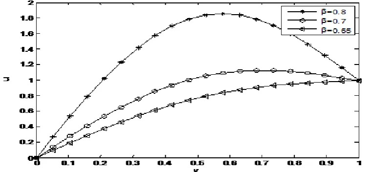
velocity u decreases. From Fig.2 it is observed that the primary velocity 𝑢𝑢(𝑦𝑦) increases with an increase in the

fractional calculus parameter β which is different from the case in Fig. 1. The effect of permeability of the porous

medium K on 𝑢𝑢(𝑦𝑦)can be observed in Fig.3. As K increases the velocity deceases that is the presence of the porous

medium resists the primary flow. The secondary flow velocity w is depicted in Fig.4 against the distance from the

stationary plate for different values of the parameter α. It is seen that the secondary flow decreases for higher values of

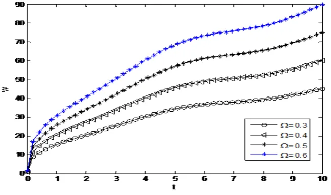
α. In Fig.5 the scenario is different. The secondary flow increases as the parameter β increases. The secondary velocity

is depicted against time t for different values of the rotation parameter Ω in Fig. 6 and from there it can be observed

that as Ω takes higher values the secondary flow increases. In Fig.7 the secondary flow increases with increase in the

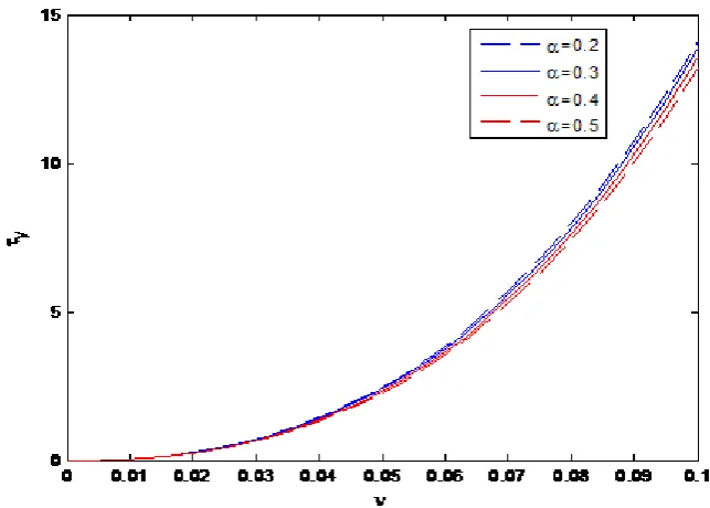
distance from the stationary plate at 𝑦𝑦= 0. The shear stresses 𝜏𝜏_𝑥𝑥 and 𝜏𝜏_𝑦𝑦 due to the primary and secondary flows are

depicted against the kinematic viscosity υ in Fig.8 and Fig.10 respectively for different values of the fractional calculus

(9)

Fig. 1: The primary velocity u is depicted against the distance from the lower plate for different values of fractional

calculus parameter α. 𝜐𝜐= 0.03,𝜆𝜆𝑟𝑟 = 3,𝑐𝑐= 0.1,Ω= 0.3,𝜎𝜎= 1,𝐵𝐵0= 5,𝜌𝜌= 0.05,𝜇𝜇= 0.04, 𝜆𝜆= 2,𝜀𝜀= .002, 𝛽𝛽= 0.8,𝐷𝐷= 1,𝐾𝐾= 1

Fig. 2: The primary velocity u is depicted against the distance from the lower plate for different values of fractional

calculus parameter β𝜐𝜐= 0.03,𝜆𝜆𝑟𝑟 = 3,𝑐𝑐= 0.1,Ω= 0.3,𝜎𝜎= 1,𝐵𝐵0= 5,𝜌𝜌= 0.05,𝜇𝜇= 0.04,𝜀𝜀= 0.02,𝜆𝜆= 2, 𝛼𝛼= 0.2,𝐷𝐷= 1,𝐾𝐾= 1

Fig. 3: The primary velocity u is depicted against the distance from the lower plate for different values of the parameter

(10)

Fig. 4: The secondary velocity is depicted against the distance from the lower Stationary plate for different values of

the parameter α. 𝜀𝜀= 0.02,𝜐𝜐= 0.03,𝜆𝜆𝑟𝑟 = 3,𝑐𝑐= 0.1,𝛺𝛺= 0.3,𝜎𝜎= 1,𝐵𝐵0= 5,𝜌𝜌= 0.05,𝜇𝜇= 0.04,𝜆𝜆= 2, 𝛽𝛽= 0.8, 𝐷𝐷= 1,𝐾𝐾= 1

Fig. 5: The secondary velocity is depicted against the distance from the lower stationary plate for different values of

the parameter β. 𝜀𝜀= 0.02,𝜐𝜐= 0.03,𝜆𝜆𝑟𝑟= 3,𝑐𝑐= 0.1,𝛺𝛺= 0.3,𝜎𝜎= 1,𝐵𝐵0= 5,𝜌𝜌= 0.05,𝜇𝜇= 0.04, 𝜆𝜆= 2, 𝛼𝛼= 0.2,𝐷𝐷= 1,𝐾𝐾= 1

Fig. 6: The secondary velocity is depicted against time for different values of the parameterΩ. 𝜀𝜀= 0.02, 𝜐𝜐=

(11)

Fig. 7: The secondary velocity is depicted against time for different values of the distance from the stationary plate 𝑦𝑦. 𝜀𝜀= 0.02,𝜐𝜐= 0.03,𝜆𝜆𝑟𝑟 = 3,𝑐𝑐= 0.1,𝛺𝛺= 0.3,𝜎𝜎= 1,𝐵𝐵0= 5,𝜌𝜌= 0.05,𝜇𝜇= 0.04,𝜆𝜆= 2,𝛼𝛼= 0.2,𝛽𝛽= 0.8,𝐾𝐾= 1

Fig. 8: The shear stress due to the primary flow is depicted against the kinematic viscosity for different values of the

(12)

Fig. 9: The shear stress due to the primary flow is depicted against the kinematic viscosity for different values of the

parameter β. 𝜀𝜀= 0.02,𝜐𝜐= 0.03,𝜆𝜆𝑟𝑟 = 3,𝑐𝑐= 0.1,𝛺𝛺= 0.3,𝜎𝜎= 1,𝐵𝐵0= 5,𝜌𝜌= 0.05,𝜇𝜇= 0.04,𝜆𝜆= 2,𝛼𝛼= 0.2, 𝐷𝐷= 1,𝐾𝐾= 1

Fig. 10: The shear stress due to the secondary flow is depicted against the kinematic viscosity for different values of

the parameter α. 𝜀𝜀= 0.02,𝜐𝜐= 0.03,𝜆𝜆𝑟𝑟 = 3,𝑐𝑐= 0.1,𝛺𝛺= 0.3,𝜎𝜎= 1,𝐵𝐵0= 5,𝜌𝜌= 0.05,𝜇𝜇= 0.04,𝜆𝜆= 2,𝛽𝛽= 0.8, 𝐷𝐷= 1,𝐾𝐾= 1

5. ACKNOWLEDGEMENT

The authors are thankful for the valuable comments of the reviewers to prepare the paper in the present form.

6. REFERENCES

[1] Bose D. and Basu U., Unsteady incompressible flow of a generalized Oldroyed-B fluid between two infinite

parallel plates World Journal of Mechanics,3(2013), 146-151

[2] Chand K. and Sharma S., Hydromagnetic oscillatory flow through a porous channel in the presence of Hall

current with variable suction and permeability, International Journal of Statistika and Mathematika, 3(2012),

70-76.

(13)

[4] Guria M., Jana R.N. and Ghosh S. K., Unsteady Couette flow in a rotating system, International Journal of Non-linear Mechanics, 41(2006), 838-843.

[5] Jana R. N. and Datta N., Couette flow and heat transfer in a rotating system, Acta. Mech., 26(1977), 301-306.

[6] Mazumder B. S., An exact solution of oscillatory coquette flow in a rotating system, ASME J. Appl. Mech., 56

(1991), 1104-1107.

[7] Prasad B. G. and Kumar R.,Unsteady hydromagnetic Couette flow through a porous medium in a rotating system,

Theoretical and Applied Mechanics Letters 1, (2011)Article ID: 042005.

[8] Singh K. D. and Sharma R., Three dimensional Couette flow through medium with heat transfer, Indian J. pure

appl. Mathematics, 31(2001), 1819-1829.