©Science and Education Publishing DOI:10.12691/amp-6-1-1
Analysis of Various NASA Satellite Images through
the Techniques of Image Morphing
Tanvir Prince1,*, Jenifer Vivar2, Fabian Ramirez1
1
Department of Mathematics of Eugenio Maria de Hostos Community College of the City University of New York, 500 Grand Concourse, Bronx, New York, 10451, United States
2
Department of Natural Sciences of Eugenio Maria de Hostos Community College of the City University of New York, 500 Grand Concourse, Bronx, New York, 10451, United States
*Corresponding author: [email protected]
Abstract
Image morphing is a technique that implements linear algebra (geometric and algebraic transformation techniques) to transform one point in a plane to the other. We analyze images through image morphing techniques to predict changes that had happened through time and also what might happen in the future. The purpose of this particular research is to observe the changes of different NASA satellite images, describe the observations, and hypothesize the possible causes of the phenomena observed in the morph. This is performed by using two satellite images. These images were taken at two different intervals of time, morph the images and observed the gradual changes of the objects. The selected pictures did not have additional documentation (for example, images between a selected interval of time) available to compare so morph was used to analyze the transition. How accurate are all these morphing techniques? The accuracy of the transformation is analyzed by taking pictures of a blooming flower and documents all the phases between the blooms. Then, the morphing technique is implemented towards the first and last picture to compare the changes previously observed in the morph. This experiment was conducted to predict the uncertainty of the transformation. Image morphing techniques are important because when satellites document images of an object at a certain time, it may take a while for another picture to be documented again. By then, many things could have changed and the purpose is to investigate how such changes occurred. The morph is an accurate approximation to the actual changes of the objects and a very useful tool to use when it is impossible to take consecutive pictures of a constantly changing place or object. Furthermore, this technique can help to discover patterns of the objects and enable scientists to hypothesize future changes. A morphing software named, Morph Age, was used to morph the pictures.Keywords
: image morphing, morph age, NASA, satellite Images, Mathematica, RGB valuesCite This Article:
Tanvir Prince, Jenifer Vivar, and Fabian Ramirez, “Analysis of Various NASA Satellite Images through the Techniques of Image Morphing.” Applied Mathematics and Physics, vol. 6, no. 1 (2018): 1-9. doi: 10.12691/amp-6-1-1.1. Introduction
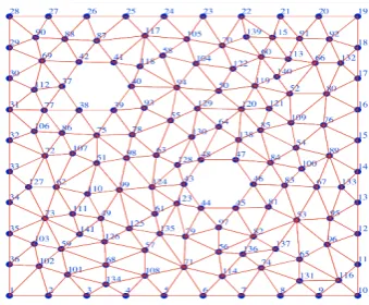
Morph is the process in which one image gradually transform into another by averaging the select points or values of the image to a final picture using transformations techniques [1,2]. The selected points are later connected into triangles then, each triangle in the image can be morphed individually. This process is known as triangulation (Figure 1). Image morphing is usually used in the TV industry to create a smooth transition effect of, said, a human becoming a monster. While this is a good technique to implement in the film and entertainment world image morphing techniques can go beyond that (White). Image morphing techniques have been used in the science field. For instance, image morphing was used to predict abnormal growth of a cell [3]. The mathematical techniques (mathematics will be briefly mention in the next section) can make very accurate predictions on how certain objects change with respect to time if this had
specifically interested in the sun spots (relatively cool areas in the sun surface) and how they have become scarce with time. And the B-34 glacier located at the Antarctic region will show us the fast way in which the polar ice caps are melting. Moreover, we also put the predictions made by the image morphing techniques by documenting the blooming of a flower and compared them with the result of the morph. The picture endorses the efficiency of the morphing techniques. Image morphing techniques can be used in diverse fields in order to predict events that were not properly documented and it is a good tool to support scientific theories or hypothesis.
Figure 1. Shows an image undergoing triangulation, it forms triangles and covers the entire image
Figure 2. Shows part of the matrix for of the picture considered as the input. Computers read the images as a matrix form of RGB values and the amount of color from zero to one
2. Mathematics behind Image Morphing
Every picture is seen by a computer as a set of values in matrix from. For instance, in Figure 2, it shows the translation of a picture translated in the language of the computer.
Each pixel has a different value to the colors red, green and blue also known as the RGB values of the image (Prince, Franco, Salva, & Windolf, 2014). Moreover, each pixel becomes an array of values for each red, green and blue colors therefore producing a matrix. When an image is morph the values of each pixel’s current RGB value need to be multiply by a scalar quantity, in other words, each value in the matrix array should be multiplied by a number representing the time between the 0 and 1 [3]. The values of the initial and final pictures are known and the picture in between the first and last becomes an average of the two. The use of applied mathematics in technology has open a window to perform task that we were not able to approach before. Linear algebra is very useful when dealing with images that need to be moved from one slide to the other. Image morphing is the techniques used to perform such tasks. Image morphing itself is the application
of linear transformation and triangulations that allowed a computer to predict an ending point. Triangulation is when several points are selected in the picture and are later connected to form triangle, Figure 3 shows an image with several points selected and then connected to form triangles, noticed that the lines do not cross each other.
The equation use for the transformation of any picture A that is transforming into a final picture C and the resultant morph image in-between, B at any given time “t” is given by the following equation:
( ) (
= −)
+ .B t 1 t A tC
Linear transformation is simply a function that takes an input and spits out an output for each value. In the case of linear algebra, it would be a transformation that takes a vector as an input and produces another vector as an output. Linear transformation are functions that keep grid lines parallel and evenly spaced. To express this numerically one would have to give a formula so when the coordinates of a vector are given we could get the coordinates of the output vector. More detailed information can be found at previous research done about image morphing [3,4].
3. Methodology
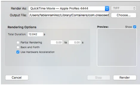
The program used to make image morphing was Morph Age for MacOS which was developed by the company, Creaceed as early as April 8th, 2003. The version that was utilized was the 2016 update known as, Morph Age 4.2.3. Morph Age can compress the image morphing in a high definition QuickTime video, which can show crystal clear detailing. The understanding of this program is simple, it does not take previous computer knowledge to get the hang of it. The benefit of Morph Age is the accuracy of pixels when using the zooming feature, which is great so that the triangulation doesn’t become visible in the final product. To use this application, there are a couple of steps that were performed:
1. Drop the two images that are being morph in their respective trays. (The first two trays are the ones being used, the third one is the final product. It shows an animation of the change.)
This is an example of how the trays would look before the placement of the image that are going to be morphed.
2. Once each picture is in their respective tray, place the “dots”, which are the morphing indicators that will make the image morph as smooth as possible. To get the best results, place the dots in every detail of the image.
3. There are five icons on the top-right hand corner of the screen; the one in the middle will be clicked on, in order to have the image time layout on the bottom of the screen. By the program’s default, both images will be set to 5 seconds. However, 5 seconds is too fast to see the gradual changes of both images. This is where one can adjust the morph time for both images.
4. Focusing on the lower part of the program, there are knobs to extend or shorten the length of the images.
5. There is a gray tab on top of the image tap that must be extended first for the image length to be extended as well. Once, the gray tab has been extended, the image can also be extended (seen in purple), it can be adjusted to whichever time one wants. In this case, the duration of the morph will be 12 seconds long. The process is the same for the second image.
4. Results
4.1. How Old Was the Last Ice Age in Mars?
According to scientist, the last ice age of Mars happened around 2.1 to 0.4 million years ago [5,6]. The planet has been analyzed for a great period due to the similarities to planet earth. According to scientists, evidence collected by the NASA's Mars Global Surveyor and Mars Odyssey missions have showed enough evidence to suggest a possible Ice age. Data shows that the surface of the planet Mars was covered by a thick layer of ice composed of carbon dioxide. The frozen carbon dioxide (dry ice) located at the poles of Mars also shows evidence of a possible previous ice age in Mars. Scientists analyzed the different layers of ice that are located at Mars’ poles and have conclude that the amount of snow that has fallen into the surface during a period seems to be different as that of recent falls3. Scientist explain that there should have been a period where snow did not stop
falling and therefore the difference between layers, the ones that are less dense represent snow fallen during different seasons as shown in Figure 4. Compared to Earth, Mars seems to also have been in between recent ice ages and a picture of its possible look was published in the scientific journal Nature [7]. The image was taken and morph with the help of the Morph Age software to try to predict the way in which Mars thawed itself and if the frozen concentrations of dry ice located at the poles are the leftovers of a recent Ice age. The image of the morphed version of the transition of the last ice age and the present time is simulated and shown in figure 4. The images show the sequence from the believe image of Mars during the last ice age to recent years. The images are in regression form in years from the last ice age till now. The sequence shows that as the planet was exiting the ice age most of the ice that was covering the planet “move” towards the poles. Perhaps this happens due to the sun’s incapability of reaching those areas, just as Earth. The changes observe in the morph agrees with what happened to earth during the last peak of the ice age we are currently on. Due to the different speed in which the red planet rotates its climate is affected by it. For instance, earth’s rotation over the last 10 million years has go from 22º to 24.5 º while Mars went from 14 º to 48 º which is almost double [6]. Moreover, one Martian year is almost double to that of earth or 687 Earth days. This could possible indicate the reasons why Mars’ Ice age is over and planet Earth is still experiencing its effects. The images obtained through the morph of Mars could be of great importance to compare the changes occurred at the end of it last Ice age. This is because planet earth is still in the middle of its last ice age and based on the data collected we can predict the way in which planet Earth will probably behave.
Figure 4. Shows the possible look of planet Mars counting how many years has pass from the last Ice age until modern times. Each year decreases from 400 kya (thousand years ago), to 40 kya
Though Earth is still under the last ice age effects, it is notorious that the concentration of ice is concentrated in the poles, evidence shows that the Antarctic for instance use to be a place where tropical plants grew. Something similar might have happen to Mars, even though they might have not been any type of life at the time the concentration of frozen zone also concentrated in the poles where huge amounts of carbon dioxide might be storage. Figure 5 in the sequence shows how ice started to disappear slowly vanishing through the ends of the poles of Mars.
4.2. Jupiter’s Great Spot
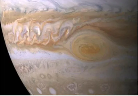
Jenifer’s Jupiter is the biggest planet of our solar system, it is 11 times wider than earth and more than a thousand earth could fit inside. Moreover, one day at Jupiter last only about 10 hours because the spin of the planet is significantly fast. The planet also takes longer to completely rotate around the sun, a year in Jupiter has 4300 days [8]. The composition of Jupiter is mostly the same as the sun, helium and hydrogen, but it also has toxic gases such as ammonia and ethane. The most notorious part of Jupiter is perhaps the red great spot or its technical name anticyclone. This was first observation during the 1600’s and it seems to not have move since then; the anticyclone is about 300 years old, or perhaps older since it was already formed by the time it was discover [9]. It is known that the wind’s speed inside the anticyclone is about 500 kilometers per hour. Scientist believe that the reason why the great red spot has not move is because of the anticyclone is a vortex, a spinning region in a fluid, and persists because the planet is rotating as well and a faster speed. The close observations of the planet show the way the red spot is moving; scientist have observed that before. In the image sequence below, the Jupiter’s Great Spot is shown to be moving across the surface. Moreover, the red spot also seems to be shrinking according to the images obtained from the morph. Figure 6 shows a beginning picture taken in 2009 and the last picture taken at 2014 and the many changes occurred to the red spot and other parts.
Figure 6. Shows a close look, into the anticyclone, or the big red spot
The red spot was observed to be losing part of its mass to the side cooling clouds of ammonia while it rotates [10]. As observed in the third and fourth time frame of Figure 7,
a white looking cloud seems to be slowly coming out of the anticyclone and fusing with the nearby belt of Jupiter (dark bands of Jupiter are called belts and the lightest ones are zones). A small amount of white clouds is observed in the beginning picture taken in 2004, however, as observed in the last picture the size of the cloud is significantly bigger. According to the observations, it is more likely that the red spot could disappear in the upcoming years. Another identify storm was that right below the red spot observed in picture one. Then as time passes the storms seemed to have moved at a faster rate from its initial position and compared to the great red spot. The reason might be because of the speed in which of the great spot is coming out of the anticyclone zone. It is likely that the gas comes out with such great force that it “pushes” the small storm far away. Furthermore, the big cloud that was in one of the planet zones seems to also be disappearing. In image one we can see the cloud located in the biggest zone of Jupiter starting big and then slowly disappear. This might be because the zone part, the lightest belts of Jupiter, is moving at a faster rate and it seems to be fusing with the belt located above it.
4.3. The Phenomenon of Sunspots
Sunspot(s) are basically the darker areas of the sun which are surprisingly cooler compared to the surrounding surface, the photosphere, temperature of the sun. The sun is generally about 9,900°F (or roughly about 5,500°C), the sunspot area can range anywhere from 4,900 – 7,600 F, (or 2,700–4,200 °C); it is roughly about 2,300 F, or 1300 C cooler from the maximum temperature of the sunspot (Spacetelescope, 2013). Since the sun is about 870,000 miles in diameter, the size of the sunspot can vary in diameter due to the large surface of the photosphere. Sunspot’s formation is due to the Sun’s magnetic field flooding the photosphere, which can take up days or weeks; however, it can last for weeks or even months. The magnetic field of the sunspot can cause solar flares and Coronal Mass Ejections, these solar activities are also called solar storms. The way these two types of storms release their energy can be that of a rubber that is being twisted until it breaks or “snaps.”
Figure 7. is an image sequence of Jupiter, specifically it showcases the red spots in Jupiter's surface moving as time goes by
Figure 8. showcases the sunspots between five different intervals of time. It starts from t=0, which is the initial of that specific time and ends in t=1, which is the conclusion of that period. The time ranges from 2008 – 2014, which is a 6-year difference. There is a gradual change in the sunspots from 2008 to 2014
In conjunction with image morphing, the purpose of this sector was to establish the understanding of different sunspot location, as well as the possible conclusion that can be determined. The analyzes takes place between a 6-year gap which starts in 2008 and ends in 2014; as an obvious visual, the sunspot both “disappears” and “reappears” throughout time. The formation of the sunspot, as stated previously, can take takes or weeks, meaning the sunspot in 2014 can be considered “fresh”, and the ease of any previous sunspot can last weeks or months. Image morphing can be useful to figure out other potential locations for the sunspots and figuring out if the magnetic field would increase, decrease or stay steady. Image morphing also provides an image that can indicate the transition of sunspots throughout time. The Figure 8 above shows the gradual change of the sunspots throughout the 6-year period, it is divided in 5 different sections of time. Each section is an estimate about a year and two months, which makes it easier to track its progress. In the initial picture, there were a couple of smaller sunspots that formed, it is scattered around the sun’s photosphere; but as time progresses the scattering “disappears” and a more darker and bigger sunspot is formed in the lower section of the picture. Darker and bigger sunspots may indicate a greater amount of magnetic field present. However, there’s been reports that show that the sunspot’s magnetic field have been declining throughout the years, the opposite of the conclusion. Since the magnetic field is declining, sunspots can also slowly cease to exist; which means not a lot of solar activities. In a way, this is beneficial for the technologies that are orbiting around space.
With the use of image morphing techniques, one can hypothesize the gradual formation of a new sunspot, and the deformation of the old. Each sunspot is in different sectors of the sun’s photosphere, each with different levels of magnetic fields that can either be harmful to the technologies, both on land and space, as well as those in
space or it can be a neutral effect. While, this hypothesize is not fully accurate, a better understanding of sunspot is vital for those involve in space expedition. There are also some debates that showcases the correlations between the numbers of sunspots and the impact on Earth’s global climate. Since there are reports of sunspots slowly becoming a thing of the past, it is better to understand any spontaneous factors that can cause a revival to sunspots and its solar activities. The magnetic field of the sunspots is slowly decreasing; while darker and bigger sunspots does not indicate a higher level of sunspots, figuring out the pattern of the magnetic field can give an insight of future potential sunspots, even if the magnetic field hits a low point.
4.4. Iceberg B-34
The iceberg, B-34, was discovered on March 6th, 2015 by the U.S. National Ice Center; this iceberg was floating directionless from the Getz Ice Shelf in the Antarctica region. The Getz Ice Shelf is part of Operation IceBridge which is a mission that is being conducted by NASA between 2009 until 2018. The main idea behind Operation Icebridge is to understand the connection between the “Polar Regions” and the global climate system. The Icebridge also collects important data will be utilize to make predictions based on the relationship of Earth’s polar ice, climate change, and the resulting sea-level rise. The relationship between B-34 and The Getz Ice Shelf is that, this specific area has experienced high levels of basal melt rates [12]. The basal melt is known to represent the source of the subglacial water in the West Antarctica region. Iceberg B-34 is about 15 nautical miles in length and about 5 nautical miles in width. The idea is to see the impact that B-34 has on climate change through the image morphing techniques since large icebergs are known to have a high impact on the Southern Ocean.
During Operation Icebridge, there were documentations of iceberg B-34 that were taken using the Moderate Resolution Imaging Spectroradiometer (or MODIS) under NASA’s Terra an Aqua satellites during specific periods of time. The two dates that are being analyzed with image morphing will be the images taken on: February 28th, 2015, and March 5th, 2015, see Figure 9. During the span of these two dates, there are some noticeable changes that have occurred. One obvious difference is the rotation of the B-34; it starts off at the initial horizontal plane and over the course of the 5 days it starts to rotate in a 90° angle. These changes backup the information that Operation Iceberg’s mission is trying to relate; the relationship between climate changes, Earth’s polar caps and climate change. Although these changes do not showcase a drastic difference between these two specific dates, there are some changes that were done due to climate change.
There is no doubt that the sea water levels are slowly increasing steadily throughout time, since many icebergs are splitting apart from larger glacier ice caps. According to Claire Parkinson, “The planet as a whole is doing what was expected in terms of warming. Sea ice as a whole is decreasing as expected, but just like with global warming, not every location with sea ice will have a downward trend in ice extent” [7] In other words, the changes viewed in the image morph layout, shows that some parts of the iceberg B-34 are slowly melting, which is part of the planet’s process of warming.
4.5. Accuracy of Image Morph
4.5.1. Lilium Candidum
With image morphing being conducted in the pervious four experiments, a final experiment was done in order to test the accuracy of the image morph. Using the lilium candidum, or the lily, an experiment of seven days was done while starting from the intial closed lily, to the end of the lily while it was blossomed, see Figure 10 and Figure 11. The blooming process is an important component since the initial and the end product of the lily can be morphed to make a artificial half point of the lily’s morph. Comparing the motped half point of the lily, and the actual documentation of the halfpoint period, it is almost alike. However, the morphed image shows a bit of flaws because of the software restriction that prevents it from morphing a third dimensional object; the software is better for a two-dimensional linear image than an image that has volume. The image sequence below show the initial and final images of the actual lily and the in between images are morphed blooming images. The accuracy test of image morph was a good experiment to be done to understand how image morph works in real life applications.
Figure 9. showcases the Iceberg, B-34, an it’s transition though the five-day time difference that it was taken. The first image (left to right) represents the initial time, t=0, middle image represents the half point, t=.5, and the end is represented by t=1. The time period of this image is from February 28th, 2015 to March 5th, 2015, roughly 5 days. The changes are noticeable between those time differences
Figure 11. is a comparison between the original half point blooming of the lily (left), and the morphed half way blooming lily (right). As one can see, the similarities are close even with some flaws. This is a close approximation
5. Limitations
In this research, there were some limitations that dealt with equipment which hinder the project from going further. The software, Morph Age, was only limited to morphing two dimensional images instead of a third-dimension image. This is necessary since morphing images in a third-dimension can allow for an accurate hypothesize since there are more details in terms of volume than a two-dimensional image. Also, Morph Age, also had some issue with rendering high definition films in order to properly display it in a bigger screen to start coming up with a hypothesizes. Another limitation with the research was the scarce numbers of satellite images that meet with the conditions for a smooth morph. The three conditions that are highly encouraged to look for before starting the image morph is: dimension, angle, and time. In dimension, the size of the image is important since Morph Age does not know how to crop images for the morph. Use of a photo software can sound like a good idea but when it is time to save the image, the pixels for the image can be lost, which results in a blurrier image. Size and pixels are important subcomponents for the dimension umbrella for the image morph to be smooth. Angle, the way a planet, or region must have the same angle for both images; a different angle can result to a rough transformation since the triangulation that is happening in the background can become obvious in the film. Obvious triangulation can interfere with prediction, for instance, if the image of interest has white details, one can assume that nothing is occurring. This is not a good thing since the triangulation can maybe block any small details because of the angle distortion. Same goes with a darker detail of the image of interest, the triangulation will make the image look rough and the details will be missing since the triangulation is in white. Lastly, time, this is an important component because the longer the two images are from their respective documentation, the more visible the changes can appear in a morph. For instance, the B-34, which was discussed earlier in the paper, had very small changes besides the rotation of the iceberg. The longer the time, the higher chances of a drastic change can be spot and analyzed. These limitations should be taken into consideration for any potential work using image morphing techniques.
6. Future Work
For further research in the techniques of image morphing, exploring another software should be noted, since another software can provide additional features that Morph Age did not provide. Exploring different planetary properties is also another idea to consider since there are numerous of things that one does not know about another planet. Further study of Jupiter, for instance, should be done since there are many more satellite images that the spacecraft, Juno, is documenting during its rotation around the planet. Understanding Mars’ ice age is important because, it can give an insight of what the future of the planet can happen; as well as relate the weather on Mars with the weather here. Also, for future work, a better understanding of the sunspot and its correlation to the Earth’s climate should be done since the magnetic field of the sun is decreasing as time goes by. Environmental work should also be conducted for further research since it can be an affordable alternative way to understand the climate and its changing that are being caused by greenhouse gasses and other detrimental things that are harming the planet. There are also other applications that image morphing can be utilized, in terms of, analyzing planetary and environmental properties, that can be done for further research.
7. Conclusion
Image morphing techniques can be a great alternative source when one is limited in terms of equipment and funding. While there are some limitation and room for improvement, image morphing can still be utilized to not only analyze but to understand the subject that undergoes this transformation. The accuracy of image morphing was conducted in order to understand how close the morph and the actual image are; the accuracy is important for the direction of any predictions that are being made with morph. Since the accuracy was close to the actual documentation, the lilium candidum experiment, the hypothesizing of other morphing subjects can also be a strong indication of what happened in between those empty time periods when no documentation occurred. The techniques of image morphing are a good stepping stone for researching and making hypothesize, as well as, being an affordable alternative when there are not a lot of funding for a project.
Acknowledgements
program. Special thanks to CUNY’s Hostos Community College for providing a space for this research to be conducted and the NASA Goddard Space Flight Center (GFSC) Office of Education for giving us this opportunity.
References
[1] Anton, H. (2010). Elementary Linear Algebra (10th ed.). John Wiley & Sons INC.
[2] Stewart, J. (2012). Stewart Calculus Early Transcendentals 8th Edition. Cengage Learning.
[3] Tanvir Prince, M. M. (2015, November 25). (J. o. Research, Producer, & Canadian Center of Science and Education) Retrieved August 1, 2017, from The Mathematics and Applications behind Image Warping and Morphing:.
[4] Prince, T., Franco, S., Salva, I., & Windolf, C. (2014). Mathematics Behind Image Compression. Journal of Student Research, 3(1), 46-62.
[5] NASA. (2016 , May 26). Sign of Martian Ice Age. Retrieved from https://mars.jpl.nasa.gov/multimedia/images/signs-of-a-martian-ice-age&s=4.
[6] James W. Head, J. F. (2003). Recent Ice Ages on Mars. Nature.
[7] Ramsayer, K. (2014, October 7). Antarctic Sea Ice Reaches New Record Maximum. Retrieved August 1, 2017, from NASA: https://www.nasa.gov/content/goddard/antarctic-sea-ice-reaches-new-record-maximum.
[8] Clements, J., & Angeli, E. (2010). Jupiter - In Depth. Retrieved from Planets - NASA Solar System Exploratio:
solarsystem.nasa.gov/planets/jupiter/indepth.
[9] Candanosa, R. M. (2015, August 26). Jupiters Great Red Spot - A Swirling Mystery. Retrieved from News - NASA Solar System Exploration:
solarsystem.nasa.gov/news/2015/08/04/jupiters-great-red-spot-a-swirling-mystery.
[10] Space, N. A. (n.d.). National Aeronautics and Space Administration. Retrieved from National Aeronautics and Space Administration: www.nasa.gov.
[11] Fies-Faither, J., & Schirmer Lockman, A. (2009, August). Beyond Penguins and Polar Bears. (N. S. Foundation, Producer) Retrieved August 21, 2017, from Ohio State University:
http://beyondpenguins.ehe.osu.edu/issue/icebergs-and-glaciers/all-about-icebergs.
[12] Hansen, K. (2016, November 9). Getting to Know the Getz Ice. NASA's Earth Observatory. Retrieved from