Vol 9, No 1 (2018)

Available online throug

ISSN 2229 – 5046

LINEAR ANALYSIS OF THERMAL INSTABILITY

IN A POROUS MEDIUM SATURATED BY MAXWELL NANOFLUID

JADA PRATHAP KUMAR*, JAWALI CHANNABASAPPA UMAVATHI**

AND CHANNAKESHAVA MURTHY***

*Department of Mathematics, Gulbarga University, Karnataka, India.

**Department of Mathematics, Gulbarga University, Karnataka, India.

***Department of Mathematics, Govt. First Grade College, Bidar, Karnataka, India.

(Received On: 06-12-17; Revised & Accepted On: 21-12-17)

ABSTRACT

I

n the present article onset of convection in a horizontal layer of porous medium saturated with a Maxwell nanofluid is studied by linear analysis. The modified Darcy-Maxell nanofluid model is used to simulate the momentum equation in porous media. The nanofluid incorporates Brownian motion and thermophoresis.A Galerkin method has been employed to investigate the stationary and oscillatory convections, the stability boundaries for these cases are approximated by simple and useful analytical expressions. To investigate the stability of the system, parameters such as Nanopartical concentration Rayleigh number, Lewis number, modified diffusivity ratio, Vadasz number and relaxation are varied. It is found that for stationary convection Lewis number and modified diffusivity ratio stabilizes the system where as Nanopartical concentration Rayleigh number and porosity destabilizes the system. For oscillatory convection the thermal capacity ratio stabilizes the system while nanopartical concentration Rayleigh number, Lewis number, porosity and vadas number destabilizes the system.

Keywords: Nanofluid, Porous medium, Natural convection Horizontal layer, Conduction and viscosity variation,

Brownian motion and thermophoresis.

Nomenclature

B

D Brownian diffusion coefficient (m s2 ), given by

T

D Thermophoretic diffusion coefficient (m s2 ),

H Dimensional layer depth (m)

k Thermal conductivity of the nanofluid (W/m K)

m

k Overall thermal conductivity of the porous medium saturated by the nanofluid K Permeability ( 2

m )

Le

Lewis number A

N Modified diffusivity ratio

B

N Modified particle density increment *

p Pressure (Pa)

p Dimensionless pressure, * f

p K µα

λ non dimensional relaxation time

Va Vadasz number

a

γ

non dimensional acceleration coefficient

T

Ra Thermal Rayleigh- Darcy number Rm Basic-density Rayleigh number Rn Concentration Rayleigh number

Corresponding Author: Channakeshava Murthy***

*

t Time (s)

t Dimensionless time, * 2 f

tα H

*

T Nanofluid temperature (K)

T Dimensionless temperature,

* *

* *

c

h c

T T T T

− −

* c

T Temperature at the upper wall (K) *

h

T Temperature at the lower wall (K)

(

u v w, ,

)

Dimensionless Darcy velocity components

(

*_, *_, *

)

m

u v w H α (m/s)

v Nanofluid velocity (m/s)

(

x y z, ,

)

Dimensionless Cartesian coordinate

(

* * *

)

, ,

x y z H;

z

is the vertically upward coordinate

(

_{x y z}*_, *_, *

)

_{Cartesian coordinates}

Greek symbols

m

α Thermal diffusivity of the porous medium

ρ Fluid density

p

ρ Nanoparticle mass density

σ

Thermal capacity ratio

*

φ Nanoparticle volume fraction

φ Relative nanoparticle volume fraction, * *

0 * *

1 0

φ φ φ φ − − µ Viscosity of the fluid

β Thermal volumetric coefficient (K-1)

v Viscosity variation parameter

ε Porosity

η Conductivity variation parameter

Superscripts

* Dimensional variable

'

Perturbed variable

Subscripts

b Basic Solution f Fluid

p Particle

1. INTRODUCTION

A wide variety of industrial process involves the transfer of heat energy. Nanofluid is a new kind of heat transfer medium containing nanoparticle (1-100nm) suspended in a base fluid which can be water or an organic solvent.

The transport properties of heat transfer can be enhanced by using nanofluid. Xuan and Li [1] reported that there is a 39% increase in the heat transfer coefficient using nanofluid containing 2% (v/v) copper nanoparticles. Wen and Ding [2] witnessed a 40% enhancement in the heat transfer coefficient for a nanoflid containing 1.25% (v/v) alumina nanoparticles.

The double diffusive convection instabilities in a horizontal porous layer was studied by Neild[3,4]. The linear stability analysis was extended by Taunton et al. [5], Tuner [6, 7]. The dissolution or precipitation of the solute effect the onset of convection was discussed by Richardson[8], Wan and Tan [9,10] study stability analysis of double diffusive convection of Maxwell fluid in a porous medium, they pointed out that the relaxation time of Maxwell fluid enhances the instability of the system. The Double diffusive convection of Oldroyd-B fluid in the porous media was studied by Malashetty [11, 12, 13].

volume fraction becomes very small. The basic solution is taken as a linear function of vertical coordinate. McKibbin and O’Sullivan [15, 16] and Leong and Lai [17, 18] studied the vertical heterogeneity (especially the case of horizontal layers). McKibbin [19], Nield [20] and Gounat and Caltagirone [21] carried out their studies to study the horizontal heterogeneity. Vadász [22], Braester and Vadász [23] and Rees and Riley [24] discussed some more general aspects of conductivity heterogeneity.

In this paper we intend to perform a linear stability analysis of a nanofluid-saturated porous medium by regarding the nanofluid as a viscoelastic fluid. The Maxwell fluid model is employed to describe the rheological behavior of the nanofluid.

2. ANALYSIS

2.1. Conservation equation

We select a coordinate frame in which the z-axis is aligned vertically upwards. We consider a horizontal porous layer saturated with a Maxwell nanofluid confined between the planes *z =0 and *z =H_{.Asterisks are used to denote}

dimensional variables (previously an asterisk has not been needed because all the variables were dimensional). Each boundary wall is assumed to be impermeable and perfectly thermally conducting. The temperatures at the lower and

upper wall are taken to be Th* and * c

T . The Oberbeck–Boussinesq approximation is employed. In the linear stability

theory being applied here, the temperature change in the fluid is assumed to be small in comparison with * c

T . The conservation equation is

*_. * ₀ D

V

∇ =

(1)

If one introduces a buoyancy force and adopts the Boussinesq approximation and uses the modified Darcy model for a porous medium saturated with a Maxwell nanofluid can be written as

(

)

*

* * *

1 * * 1 *

1 D 1 eff

D

V

p g K

t t t

µ ρ

λ λ ρ

ε  ∂  ∂ ∂  ₊  ₌ ₊  _{−∇ + −}    _∂  _∂  _∂ 

     v (2)

The thermal energy equation for a nanofluid can be written as

( )

*

( )

* * *

(

*2 *

)

( )

* * * * * * * *

* . * .

T

D m B

m f p

C

D T

c c T k T c D T T T

t T

ρ ∂ + ρ ∇ = ∇ +ε ρ _ ∇φ ∇ +_ _∇ ∇ _

∂ v _{   }

(3)

*

* * * *2 * *2 *

* * 1 . T D B C D D T t T

φ _{ϕ φ}

ε

 

∂

+ ∇ = ∇ +_{ }∇

∂ v _{ } (4)

we write * ₍ *_, *_, *₎ D = u v w

v .

We assume that the temperature and the volumetric fraction of the nanoparticles are constant on the boundaries. Thus the boundary conditions are

* * * * * *

0

0, _h, 0

w = T =T φ =φ at z =

(5)

* * * * * *

1 0, _C,

w = T =T φ =φ at z =H

(6)

We recognize that our choice of boundary conditions imposed on φ* _{is somewhat arbitrary. It could be argued that zero} particle flux on the boundaries is more realistic physically, but then one is faced with the problem that it appears that no steady-state solution for the basic conduction equations is then possible, so that in order to make analytical progress it is necessary to freeze the basic profile forφ*, and at that stage our choice of boundary conditions is seen to be quite realistic.

We introduce dimensionless variables as follows. We define

* * * * 2

( , , )x y z =(x y z, , ) /H t, =tα σ_m/ H

* * * *

( , , )u v w =(u v w H, , ) /α_m, p= p K/µα_m

* * * *

0

* * * *

1 0

, C,

h C T T T T T φ φ φ φ φ − − = = − − (7)

where , ( )

( ) ( )

p m m

m

p f p f

Then Eq (1)-(6) take the form

. 0

∇ =v ₍₉₎

ˆ ˆ ˆ

1 a p Rm z Ra TT z Rn z 0

t t

λ ∂ γ ∂ φ µ

 ₊  _{+ ∇ + − +} _{+ =}

 _∂  _∂ 

  

v

e e e v

(10)

2

. NB . N NA B .

T

T k T T T T

t Le φ Le

∂

+ ∇ = ∇ + ∇ ∇ + ∇ ∇

∂ v  (11)

2 2

1 1 1

. NA _T

t Le Le

φ _{φ φ}

σ ε

∂

+ ∇ = ∇ + ∇

∂ v (12)

0 , 1, 0 0

w= T = φ= at z= (13)

0, 0, 1 1

w= T = φ= at z= (14)

Here m

B Le D α = , * T m

g KH T Ra ρ β

µα ∆

= , [ p 0 (1 0)]

m

gKH Rm ρ φ ρ φ

µα

∗_{+ −} ∗

= ,

* *

1 0

( p )( )

m

gKH Rn ρ ρ ϕ ϕ

µα − − = , A N = * * * 1 0 , ( ) T B c D T D T φ∗ φ

∆

− NB=

* 1 0 ( ) ( ) ( ) p f c c ε ρ ϕ ϕ ρ

∗_{− ,µ} µeff

µ =

 , 1

2 m H λ α λ σ

= , _a

Va ε γ σ = , 2_Pr Va Da ε

= , Pr

m µ ρα = , 2 K Da H =

The relaxation parameter is a dimensionless number used in reheology to characterize how fluid and material are. The smaller the relaxation parameter, the more fluid the material appears. The parameter λ that relates to the relaxation time to the thermal diffusion time is of order one for most viscoelastic fluids. The value for relaxation parameter for dilute polymeric solution is most likely in the ranged [0.1,2]. The Prandtl number affects the stability of the porous system through the combined dimensionless group know as Vadasz number. The Vadasz number is also known as Darcy-Prandtl number in the literature. Eq (10) has been linearized by neglecting a term proportional to the product of

π and T. This assumption is likely to be valid in the case of small temperature gradients in a dilute suspension of nanoparticles.

2.2. Basic solution

We seek a time-independent quiescent solution of Eq (9)–(12) with temperature and nanoparticle volume fraction varying in the z-direction only that is a solution of the form

v

=0, T=

T

_b (z),

φ =

φ

_b(z) ,p= p z_b( )

Eq (11) and (12) reduce to 2

2 2

.

( ) 0

b B b b A B b

d T N d dT N N dT Le dz dz Le dz dz

φ

+ + = (15)

2 2

2 0

b b

A

d d T

N dz dz

φ

+ = (16)

Using the boundary conditions (13) and (14)

(1 )

b N TA b NA Z NA

φ = − + − + (17) and substitution of this in to Eq (15) gives

2

2

(1 )

0

b A B b

d T N N dT

Le dZ

dZ

−

+ = (18)

The solution of Eq (18) satisfying Eq (13) and (14) is (1 ) (1 )/

(1 ) / 1

1

A B A B

N N Z Le

b N N Le

e T e − − − − − − =

− (19)

The remainder of the basic solution is easily obtained by first substituting in Eq (23) to obtain φ_b and then using

integration of Eq (10) to obtainP_b.

According to Buongiorno[25], for most nanofluids investigated so far Le/(

φ

₁∗

−

φ

₀∗) is large, of order

10

5–

10

6, and since the nanoparticle fraction decrement is typically no smaller than

10

3this means so that Le is large, of order

2

z

T

_b

=

1

−

(20) and so ϕ =_b z

(21)

2.3. Perturbation solution

We now superimpose perturbations on the basic solution. We write

' =

v v ,p=pb+p',T= +Tb T',ϕ ϕ ϕ= b+ ' (22) Substitute in Eq (9)–(12), and linearize by neglecting products of primed quantities. The following equations are obtained when Eq (20) and (21) are used.

. ' 0

∇v = (23)

ˆ ˆ ˆ

1 p _a Ra T_{T z} Rm _z Rn _z 0

t t

λ ∂ γ ∂ ′ φ µ

 ₊ _{∇ +′ − ′ + + ′} _{+ ′=}

 _∂  _∂ 

  

v

e e e v (24)

2 2

' ' ' '

' ' NB N NA B

T T T

w k T

t Le z z Le z

ϕ

∂ _{− = ∇ +} ∂ ₋∂ ₋ ∂

 

∂   ∂ ∂  ∂ (25)

2 2

1 ' 1 1

' ' NA '

w T

t Le Le

ϕ _ϕ

σ ε

∂ _{+ = ∇ + ∇}

∂ (26)

' 0

w = ,T'=0,ϕ'=0 at

z

=

0

and at

z

=

1

(27) It will be noted that the parameter Rm is not involved in these and subsequent equations. It is just a measure of the basic static pressure gradient.

The six unknowns u', v', w', p',T' ,ϕ' can be reduced to three by operating on Eq (24) with

e

ˆ

_zcurl curl and using

the identity curl curl

≡

grad div -

∇

2 together with Eq (23).

The result is

(

)

( )

{

}

2

(

)

{

2 2

}

1+λs sγ_a+µ z ∇ w'= +1 λs Ra_T∇_HT'−Rn∇_Hφ' (28)

here

∇

2_H is the two-dimensional Laplacian operator on the horizontal plane.

The differential Eq (25)-(28) and boundary conditions constitute a linear boundary-value problem that can be solved using the method of normal modes.

We write

( ', ', ')w T ϕ =[W z( ), ( ),Θ z Φ( )]exp(z st+ilx+imy) (29) and substitute into the differential equations to obtain

( ) (

)

{

₁

}

₍ 2 2₎

(

₁

)

2

(

₁

)

2 ₀

a T

z s s D W s Ra s Rn

µ + +λ γ −α + +λ α Θ − +λ α Φ = (30)

(

2 2

)

2 .

( ) NA N NA B NB 0

W k z D D D s D

Le Le Le

α

 

+_ − + − − Θ −_ Φ =

  (31)

2 2 2 2

1 1

( ) ( ) 0

A

N s

W D D

Le α Le α

ε σ

 

− − Θ −_ − − _Φ =

  (32)

0 , 0 , 0 0 1

W = Θ = Φ = at Z= and at Z= (33) Where

d D

dz

≡ and

α

2

=

(

l

2

+

m

2

)

1/2 (34)

Thus

α

is a dimensionless horizontal wave number.

For neutral stability the real part of s is zero. Hence we now write

s

=

i

ω

, where

ω

is real and is a dimensionless frequency.

We now employ a Galerkin-type weighted residuals method to obtain an approximate solution to the system of Eq. (30)–(32). We choose as trial functions (satisfying the boundary conditions)

, , ; 1, 2, 3...

p p p

W Θ Φ p= (35)

write W= 1

, N

p p p

A W =

∑

1 N

p P p

B =

Θ =

∑

Θ ,

1 N

p p p

C =

substitute into Eq (30)–(32), and make the expressions on the left-hand sides of those equations (the residuals) orthogonal to the trial functions, there by obtaining a system of 3N linear algebraic equations in the 3N unknowns

, , , 1, 2,...

p p p

A B C p= N. The vanishing of the determinant of coefficients produces the eigen value equation for the system. One can regardRa_Tas the eigenvalue. Thus Ra_Tis found in terms of the other parameters Trial function

satisfying the above boundary condition can be chosen as sin ; 1, 2, 3...

p p p

W = Θ = Φ = p z pπ =

In the present case, where viscosity and conductivity variations are incorporated, the critical wave number is unchanged and the stability boundary becomes

(

)

(

(

)

)

(

)

(

)(

)

(

)

2 2

2

1

1 1 1 1

1

A

T a

Rn N

J s Rn

Ra s s J J s J s s J s

J s Le Le

s Le

α α

γ λ λ λ

σ ε

λ α

σ

   

= _ + + _ + _ + − + + − + _

     

+ _ + _

 

where J=π2+α2

3. LINEAR STABILITY ANALYSIS

3.1 Stationary mode

For the validity of principle of exchange of stabilities (i.e., steady case), we have s=0

(

i e s. . = +sr isi =sr = =si 0

)

at

the margin of stability. For a first approximation we take N=1. Then Rayleigh number at which marginally stable steady mode exists becomes.

2 2 2

2

( )

T A

Le

Ra π α Rn N

ε α

+  

= − _ + _

 . (37)

Finding the minimum as α varies results in

2 4

T A

Le Ra π Rn N

ε

 

= − _ + _

 . (38)

with the minimum being attained at

α

=

π

.

We recognize that in the absence of nanoparticles we recover the well-known result that the critical Rayleigh number is equal to 4

π

2. Usually when one employs a single-term Galerkin approximation in this context one gets an overestimate by about 3% (e.g. 1750 instead of 1708 in the case of the standard Bénard problem) but in this case the approximation happens to give the exact result.

3.2 Oscillatory Convection.

We now set s=iω where ω=Im

( )(

ω ωr =0

)

in Eq (37) and clear the complex quantities from the denominator to

obtain

1 2

T

Ra = ∆ + ∆iω

For oscillatory onset ∆ =₂ 0

(

ωi ≠0

)

and this gives a dispersion relation of the form (on dropping the subscripti)

( )

₂ 2

( )

₂

1 2 3 0

b ω +b ω +b = (39)

Now Eq (39) with ∆ =₂ 0 gives

(

2

)

1 2

T o

Ra =a a +ω a (40)

Where b b₁, ₂and b₃ and a a₀, ₁ and a₂ and ∆₁and∆₂ are not presented for brevity.

We find the oscillatory neutral solution. It proceeds as follows. First determine the number of positive solution of (40). If there are none, then the minimum (over _a2 _{) with} ω2 _{given by Eq (40) gives the oscillatory neutral Ralyeigh} number. Since Eq (30) is quadratic in ω2_{, it can give rise to more than one positive value of} ω2_{, it can give rise to} more than one positive value of ω2 _{for fixed value of the parameters}

, , A,

Rn Ln N σandλ. However, our numerical

3.3 Heat and Nanoparticle Concentration Transport

The thermal Nusselt number, Nu t_f( )is defined as

( )

( )

f

Heat transport by conduction convection Nu t

Heat transport by conduction

+

=

(41)

2 /

0 2 /

0 0

( ) 1

( )

a

a B

z

T dx Z

T dx z π

π

=

 ∂ 

 _∂ 

 

= +_{ }

∂

 

∂

 

 

∫

∫

(42)

Substituting expressions (20) and (21) in Eq (42) we get

3 ( ) 1 2 ( ) f

Nu t = − πA t (43)

The nanoparticle concentration Nusselt number, Nu_φ(t) is defined similar to the thermal Nusselt number. Following the procedure adopted for arriving at Nu(t), one can obtain the expression for Nuφ(t) in the form

5 3

( ) (1 2 ( )) _A(1 2 ( ))

Nu t_φ = − πA t +N − πA t (44)

0 2 4 6 8

0 40 80 120 160

(a)

Rn = 0.01 0.05

α

Ra_T

ε = 0.9, Le = 200,

N_A = -5,

0.1

0 2 4 6 8

0 40 80 120 160

(b)

Le = 50 200 100

Le = 500

α ε = 0.9, Rn = -0.1,

N_A = -5

Ra_T

0 2 4 6 8

60 65 70 75 80

(c)

Ra_T

α

N_A = -10, -5, 0, 5, 10

ε = 0.9, Le = 200,

Rn = -0.1,

0 2 4 6 8

0 40 80 120 160

(d)

ε = 0.9, 1

ε = 0.5

α

Ra_T

N_A = -5, Rn = -0.1,

Le = 200,

ε = 5, 10, 15

2 4 6 8 1

2 3 4 5

(a)

Le=50,σ=10,ε=1,N_A=4

λ=0.5,Va=10

Ra_T Rn = -0.01,-0.02,-0.03,-0.04

α 1.5 3.0 4.5 6.0 7.5 9.0

1 2 3 4 5 6 (b)

Rn=-0.1,σ=10,ε=1,N_A=4

λ=0.5,Va=10

α

Ra_T

Le= 100,200,300,400

1.5 3.0 4.5 6.0 7.5

0 10 20 30 40

σ=1,10,20,30 (d)

α Ra_T

Le=50,ε=1,N_A=4,Rn=-0.1 λ=0.5,Va=10

2 4 6 8 10

0 2 4 6 8

(e)

Le=50,Rn=-0.1,σ

=10,ε=1

N

_A

=4,λ

=0.5,

α

Ra

_T

Va= 10,15,20,50,100

Figure-2: Neutral curves on oscillatory convection for different values of (a) nanoparticle concentration Rayleigh number Rn(b) Lewis number Le(d) porsity

ε

(d) thermal capacity ratio (e)Vadasz number Va

2 4 6 8 10

3 6 9 12 15 18 21 24 27

(c)

ε=0.1 ε=0.05 ε=0.01

α Ra_T

0.0 0.2 0.4 0.6 0.8 1.00

1.05 1.10 1.15 1.20 1.25 1.30 1.35

(a)

4 Rn=3

Le=50,N_A=5

λ=0.5,Va=10

Nu

t 0.0 0.2 0.4 0.6 0.8

1.00 1.05 1.10 1.15 1.20 1.25

(b)

100

t Nu

Le=50

Rn=4,N_A=5

λ=0.5,Va=10

0.0 0.2 0.4 0.6 0.8

1.00 1.05 1.10 1.15 1.20 1.25

(c)

5

t Nu

N_A=4

Rn=4,Le=50,

λ=0.5,Va=10

0.0 0.2 0.4 0.6 0.8

1.00 1.05 1.10 1.15 1.20 1.25 1.30

(d)

20

Rn=4,Le=50, N_A=5,λ=0.5

Va=10

t Nu

0.0 0.2 0.4 0.6 0.8

1.00 1.05 1.10 1.15 1.20 1.25

0.5

(e)

t Nu

λ=0.3

Rn=4,Le=50, N_A=5,Va=10

0.0 0.2 0.4 0.6 0.8 6

8 10 12 14

(a)

4 Rn=1

t Sh

Le=100,N_A=5

λ=0.5,Va=10

0.0 0.2 0.4 0.6 0.8

6 8 10 12 14

(b)

100 Le=50

t Sh

Rn=4,N_A=5

λ=0.5,Va=10

0.0 0.2 0.4 0.6 0.8

4 6 8 10 12 14

(c)

5

N_A=4

Rn=4,Le=100 λ=0.5,Va=10

Sh

t 40.0 0.2 0.4 0.6 0.8

6 8 10 12 14

(d)

20 _Va=10

Rn=4,Le=100 λ=0.5,N_A=5

t Sh

0.0 0.2 0.4 0.6 0.8

4 6 8 10 12 14

(e)

Rn=4,Le=100 Va=10,N_A=5

0.5

λ=0.3

t Sh

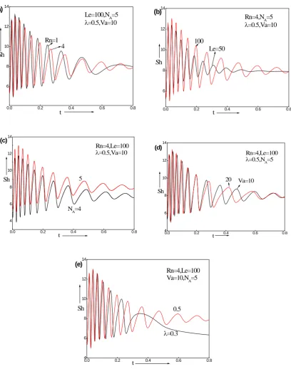
Figure-4: Variation of Sherwood number Sh with time for different values of (a) Nanoparticle concentration Rayleigh number Rn,(b) Lewis number Le, (c) Modified diffusivity ratio N_A (d) Vadasz number Va (e) relaxation time λ

RESULT AND DISCUSSIONS

Fig.1a-d shows the effect of various parameters on the neutral stability curves for stationary convection for Rn = -0.1,

Le = 200, N_A = -5,

ε

= 0.9, with variation in one of the parameters. The effect of nanoparticle concentration Rayleigh number Rn is shown in Fig. 1a. It is shown that the thermal Rayleigh number decreases with increase in nanoparticle concentration Rayleigh number Rn, which shows that nanoparticle concentration Rayleigh number Rn destabilizes the system. It should be noted that the negative value of Rn indicates a bottom-heavy case, while a positive value indicates a top-heavy case. The effect of Lewis number Le on the thermal Rayleigh number is shown in Fig. 1b. One can see that the thermal Rayleigh number increases with increase in Lewis number, indicating that the Lewis number stabilizes the system. The effect of modified diffusivity ratio N_A on the thermal Rayleigh number is shown in Fig. 1c, it is shown in

Fig. 1c that as N_A increases Ra_T increases and hence N_A has a stabilizing effect on the system. From Fig. 1d, one can

Figure 2a-e displays the variation of thermal Rayleigh number for oscillatory convection with respect to various parameters. In Fig 2a it is seen that for negative values of Rn (bottom heavy case). The thermal Rayleigh number decreases as Rn increases which will delay the onset of convection. As the Lewis number Le increases the thermal Rayleigh number Ra_T decreases as seen in Fig. 2b which imply that Lewis number Le destabilizes the system. From the picture 2c, one can reveal that the porosity

ε

destabilizes the system for oscillatory convection, that is an increase in

ε

decreases the thermal Rayleigh number. As the thermal capacity ratio

σ

increases, the thermal Rayleigh number also increases as can be observed in Fig 2d, which implies that

σ

has a stabilizing effect on the system for oscillatory convection. The effect of Vadasz number Va on thermal Rayleigh number is depicted in Fig 2e. from this figure one can see that as Va increases the thermal Rayleigh number decreases thus Va destabilizes the system.

Fig 3a depicts the transient nature of Nusselt number on nanoparticle concentration Rayleigh number Rn. It is observed that as Rn increases Nu decreases showing a decrease in the heat transport. Form Fig 3b as Lewis number increases the Nu decreases indicating there is retardation on heat transport. In Fig 3c and d modified diffusivity ratio and Vadasz number enhance the heat transport. Fig 3e shows the effect of the viscoelastic parameter λ here we find that with an increase in λ there is an increase in heat transfer, which is similar to the result observed by J.C Umavati et.al [26].

From Fig 4a and d show that as nanoparticle concentration Rayleigh number Rn and Vadasz number increases the Sherwood number decreases this show suppression of mass transport. From Fig 5b and e shows the mass transport is enhanced for Lewis number and modified diffusivity ratio. In Fig 3e we find that that as viscoelastic parameter λ increases the mass transfer increases, which are similar to the result observed by J.C Umavati et.al [26].

CONCLUSIONS

We consider linear stability analysis in a horizontal porous medium saturated with a Maxwell nanofluid heated from below and cooled from above, using modified Darcy-Maxwell model which incorporates the effects of Brownian motion along thermophoresis Linear analysis has been made using normal mode technique. We draw the following conclusions.

(1) For stationary convection Lewis number Le and modified diffusivity ratio N_A have stabilizing effect while nanoparticle concentraton Rayleigh number Rn and porosity

σ

_{destabilizes the system.}

(2) For oscillatory convection thermal capacity ratio stabilize the system while nanoparticle concentration Rayleigh number Rn, Lewis number Le, porosity

σ

and Vadasz number Va destabilize the system.

(3) The effect of time on transient number and Sherwood number is found to be oscillatory when t is small. However when t becomes very large both the transient Nusselt and Sherwood values approach to their steady state value.

REFERENCES

1. Xuan, Y. M. and Li, Q. Investigation on convective heat transfer and flow features of nanofluids,. J Heat Tran-Trans ASME, 125 (2003), 151-155.

2. Wen, D. S. and Ding, Y. L. Experimental investigation into the pool boiling heat transger of aqueous based gamma-alumina nanofluids, J. Nanopart Res., 7 (2005), 265-274.

3. Nield D. Onset of thermohaline convection in a porous medium. Water Resour. Res 4 (1968), 553-560. 4. Neild D., Bejan A., Convection in porous Media r ed, New York, Springer, (2006).

5. Taunton J, Lightfoot. E, Green T. The rmohaline instability and salt fingers in a porous medium. Phy Fluids 15 (1972), 748-753.

6. Turner J. Buoyancy Effects in fluids, London Cambridge University press, 1973. 7. Turner J. Muticomponent convection Ann. Rev. Fluid Mech 17 (1985), 11-44.

8. Rrichard.D, Richardson. C. the effect of temperature dependent solubility on the onset of themosolutal convection in a horizontal porous layer. J Fluid Mech 5 571. 59-95.2007.

9. Wang S Tan W. Stability analysis of double diffusive convection of Maxwell fluid in a porous medium heated from below. Phy Lett.A 372:3046-3050, 2008.

10. Wang S, Tan W stability analysis of soret-driven double diffusive convection of Maxwell fluid in a porous medium. Int J. Heat Fluid Flow 32 (2011), 88-94.

11. Malashety.M, Shivakumara. I, Kulkarni. S. The onset of convection in acouple stress fluid saturated porous layer using a thermal non-equilibrium mode. Phys Lett.A 373 (2009), 781-790.

12. Malashety.M, Shivakumara. I, Kulkarni. S. The onset of Lapwood-Brinkam convection using a thermal non-equilibrium model. Int J. Heat Mass Tran.48 (2005), 1155-1163.

13. Malashetty.M , Hill.A, Swamy M. Double diffusive convection in a viscoelastic fluid- saturated porous layer using a thermal non-equilibrium model Acta Mech. 223(2006), 967-983.

15. McKibbin, R, O’Sullivan, M. J. Onset of convection in a layered porous medium heated from below, Journal of Fluid Mechanicsm, vol. 96 (1980), 375-393.

16. McKibbin, R, O’Sullivan, M. J. Heat transfer in a layered porous medium heated from below, Journal of Fluid Mechanics, 111 (1981) , 141-173.

17. Leong, J. C. and Lai, F. C. Effective permeability of a layered porous cavity,. ASME Journal of Heat Transfer, 123 (2001), 512-519.

18. Leong, J. C. and Lai, F. C. Natural convection in rectangular layers porous cavities, Journal of Thermophysics and Heat Transfer, 18 (2004), 457-463.

19. McKibbin, R. Heat transfer in a vertically-layered porous medium heated from below, Transp. Porous Media, 1 (1986), 361-370.

20. Nield, D. A. Convective heat transfer in porous media with columnar structures. Transp. Porous Media, 2 (1987), 177-185.

21. Gounot J and Caltagirone J. P. Stabilite et convection naturelle au sein d’une couche poreuse non homogene., Int. J. Heat Mass Transf., 32 (1989), 1131-1140.

22. Vadász, P. Bifurcation phenomena in natural convection in porous media. In: Heat Transfer, Hemisphere, Washington, DC. 5 (1990), 147-152.

23. Braester C and Vadász P. The effect of a weak heterogeneity of a porous medium on natural convection, Journal of Fluid Mechanics, 254 (1993), 345-362.

24. Rees, D. A. S. and Riley, D. S. The three-dimensionality of finite-amplitude convection in a layered porous medium heated from below, Journal of Fluid Mechanics, 211 (1990), 437-461.

25. Buongiorno, J. Convective transport in nanofluids. ASME J. Heat Transf. 128 (2006), 240–250.

26. Umavathi,J.C., Monica .B. Mohite. Convective transport in a porous medium layer saturated with a Maxwell nanofluid. Journal of King Saud University – Engineering Sciences. 28 (2016), 56-68.

Source of support: Nil, Conflict of interest: None Declared.